AWS Machine Learning Blog

Building a customized recommender system in Amazon SageMaker

Recommender systems help you tailor customer experiences on online platforms. Amazon Personalize is an artificial intelligence and machine learning service that specializes in developing recommender system solutions. It automatically examines the data, performs feature and algorithm selection, optimizes the model based on your data, and deploys and hosts the model for real-time recommendation inference. However, if you need to access trained models’ weights, you may need to build your recommender system from scratch. In this post, I show you how to train and deploy a customized recommender system in TensorFlow 2.0, using a Neural Collaborative Filtering (NCF) (He et al., 2017) model on Amazon SageMaker.

Understanding Neural Collaborative Filtering

A recommender system is a set of tools that helps provide users with a personalized experience by predicting user preference amongst a large number of options. Matrix factorization (MF) is a well-known approach to solving such a problem. Conventional MF solutions exploit explicit feedback in a linear fashion; explicit feedback consists of direct user preferences, such as ratings for movies on a five-star scale or binary preference on a product (like or not like). However, explicit feedback isn’t always present in datasets. NCF solves the absence of explicit feedback by only using implicit feedback, which is derived from user activity, such as clicks and views. In addition, NCF utilizes multi-layer perceptron to introduce non-linearity into the solution.

Architecture overview

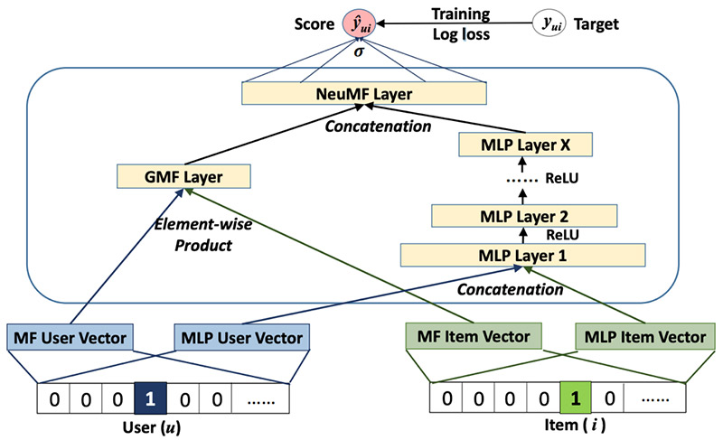
An NCF model contains two intrinsic sets of network layers: embedding and NCF layers. You use these layers to build a neural matrix factorization solution with two separate network architectures, generalized matrix factorization (GMF) and multi-layer perceptron (MLP), whose outputs are then concatenated as input for the final output layer. The following diagram from the original paper illustrates this architecture.

In this post, I walk you through building and deploying the NCF solution using the following steps:

  1. Prepare data for model training and testing.
  2. Code the NCF network in TensorFlow 2.0.
  3. Perform model training using Script Mode and deploy the trained model using Amazon SageMaker hosting services as an endpoint.
  4. Make a recommendation inference via the model endpoint.

You can find the complete code sample in the GitHub repo. You can also launch this solution in your Amazon SageMaker Studio via Amazon SageMaker JumpStart using the button below.

Open the console to get started.

Preparing the data

For this post, I use the MovieLens dataset. MovieLens is a movie rating dataset provided by GroupLens, a research lab at the University of Minnesota.

First, I run the following code to download the dataset into the ml-latest-small directory:

%%bash  
# delete the data directory if it already exists  
rm -r ml-latest-small  
  
# download movielens small dataset  
curl -O http://files.grouplens.org/datasets/movielens/ml-latest-small.zip  
  
# unzip into data directory
unzip ml-latest-small.zip  
rm ml-latest-small.zip  

I only use rating.csv, which contains explicit feedback data, as a proxy dataset to demonstrate the NCF solution. To fit this solution to your data, you need to determine the meaning of a user liking an item.

To perform a training and testing split, I take the latest 10 items each user rated as the testing set and keep the rest as the training set:

def train_test_split(df, holdout_num):  
    """ perform training testing split 
     
    @param df: dataframe 
    @param holdhout_num: number of items to be held out per user as testing items 
     
    @return df_train: training data
    @return df_test testing data
     
    """  
    # first sort the data by time  
    df = df.sort_values(['userId', 'timestamp'], ascending=[True, False])  
      
    # perform deep copy to avoid modification on the original dataframe  
    df_train = df.copy(deep=True)  
    df_test = df.copy(deep=True)  
      
    # get test set  
    df_test = df_test.groupby(['userId']).head(holdout_num).reset_index()  
      
    # get train set  
    df_train = df_train.merge(  
        df_test[['userId', 'movieId']].assign(remove=1),  
        how='left'  
    ).query('remove != 1').drop('remove', 1).reset_index(drop=True)  
      
    # sanity check to make sure we're not duplicating/losing data  
    assert len(df) == len(df_train) + len(df_test)  
      
    return df_train, df_test  

Because we’re performing a binary classification task and treating the positive label as if the user liked an item, we need to randomly sample the movies each user hasn’t rated and treat them as negative labels. This is called negative sampling. The following function implements the process:

def negative_sampling(user_ids, movie_ids, items, n_neg):  
    """This function creates n_neg negative labels for every positive label 
     
    @param user_ids: list of user ids 
    @param movie_ids: list of movie ids 
    @param items: unique list of movie ids 
    @param n_neg: number of negative labels to sample 
     
    @return df_neg: negative sample dataframe 
     
    """  
      
    neg = []  
    ui_pairs = zip(user_ids, movie_ids)  
    records = set(ui_pairs)  
      
    # for every positive label case  
    for (u, i) in records:  
        # generate n_neg negative labels  
        for _ in range(n_neg):  
            j = np.random.choice(items)  
            # resample if the movie already exists for that user  
            While (u, j) in records:  
                j = np.random.choice(items)  
            neg.append([u, j, 0])  
              
    # convert to pandas dataframe for concatenation later  
    df_neg = pd.DataFrame(neg, columns=['userId', 'movieId', 'rating'])  
      
    return df_neg  

You can use the following code to perform the training and testing splits, negative sampling, and store the processed data in Amazon Simple Storage Service (Amazon S3):

import os  
import boto3  
import sagemaker  
import numpy as np  
import pandas as pd  
  
# read rating data    
fpath = './ml-latest-small/ratings.csv'    
df = pd.read_csv(fpath)    
    
# perform train test split    
df_train, df_test = train_test_split(df, 10)    
   
# create 5 negative samples per positive label for training set    
neg_train = negative_sampling(    
    user_ids=df_train.userId.values,     
    movie_ids=df_train.movieId.values,    
    items=df.movieId.unique(),    
    n_neg=5    
)    
    
# create final training and testing sets    
df_train = df_train[['userId', 'movieId']].assign(rating=1)    
df_train = pd.concat([df_train, neg_train], ignore_index=True)    
    
df_test = df_test[['userId', 'movieId']].assign(rating=1)    
  
# save data locally first    
dest = 'ml-latest-small/s3'    
!mkdir {dest}  
train_path = os.path.join(dest, 'train.npy')    
test_path = os.path.join(dest, 'test.npy')    
np.save(train_path, df_train.values)    
np.save(test_path, df_test.values)    
    
# store data in the default S3 bucket  
sagemaker_session = sagemaker.Session()  
bucket_name = sm_session.default_bucket()  
print("the default bucket name is", bucket_name)  
  
# upload to the default s3 bucket
sagemaker_session.upload_data(train_path, key_prefix='data')    
sagemaker_session.upload_data(test_path, key_prefix='data')    

I use the Amazon SageMaker session’s default bucket to store processed data. The format of the default bucket name is sagemaker-{region}{aws-account-id}.

Coding the NCF network

In this section, I implement GMF and MLP separately. These two components’ input are both user and item embeddings. To define the embedding layers, we enter the following code:

def _get_user_embedding_layers(inputs, emb_dim):  
    """ create user embeddings """  
    user_gmf_emb = tf.keras.layers.Dense(emb_dim, activation='relu')(inputs)  
    user_mlp_emb = tf.keras.layers.Dense(emb_dim, activation='relu')(inputs)  
    return user_gmf_emb, user_mlp_emb  
  
def _get_item_embedding_layers(inputs, emb_dim):  
    """ create item embeddings """  
    item_gmf_emb = tf.keras.layers.Dense(emb_dim, activation='relu')(inputs)  
    item_mlp_emb = tf.keras.layers.Dense(emb_dim, activation='relu')(inputs)  
    return item_gmf_emb, item_mlp_emb  

To implement GMF, we multiply the user and item embeddings:

def _gmf(user_emb, item_emb):  
    """ general matrix factorization branch """  
    gmf_mat = tf.keras.layers.Multiply()([user_emb, item_emb])  
    return gmf_mat  

The authors of Neural Collaborative Filtering show that a four-layer MLP with 64-dimensional user and item latent factor performed the best across different experiments, so we implement this structure as our MLP:

def _mlp(user_emb, item_emb, dropout_rate):  
    """ multi-layer perceptron branch """  
    def add_layer(dim, input_layer, dropout_rate):  
        hidden_layer = tf.keras.layers.Dense(dim, activation='relu')(input_layer)  
        if dropout_rate:  
            dropout_layer = tf.keras.layers.Dropout(dropout_rate)(hidden_layer)  
            return dropout_layer  
        return hidden_layer  
  
    concat_layer = tf.keras.layers.Concatenate()([user_emb, item_emb])  
    dropout_l1 = tf.keras.layers.Dropout(dropout_rate)(concat_layer)  
    dense_layer_1 = add_layer(64, dropout_l1, dropout_rate)  
    dense_layer_2 = add_layer(32, dense_layer_1, dropout_rate)  
    dense_layer_3 = add_layer(16, dense_layer_2, None)  
    dense_layer_4 = add_layer(8, dense_layer_3, None)  
    return dense_layer_4  

Lastly, to produce the final prediction, we concatenate the output of GMF and MLP as the following:

def _neuCF(gmf, mlp, dropout_rate):  
    """ final output layer """  
    concat_layer = tf.keras.layers.Concatenate()([gmf, mlp])  
    output_layer = tf.keras.layers.Dense(1, activation='sigmoid')(concat_layer)  
    return output_layer  

To build the entire solution in one step, we create a graph building function:

def build_graph(user_dim, item_dim, dropout_rate=0.25):  
    """ neural collaborative filtering model  
     
    @param user_dim: one hot encoded user dimension 
    @param item_dim: one hot encoded item dimension 
    @param dropout_rate: drop out rate for dropout layers 
     
    @return model: neural collaborative filtering model graph 
     
    """  
  
    user_input = tf.keras.Input(shape=(user_dim))  
    item_input = tf.keras.Input(shape=(item_dim))  
  
    # create embedding layers  
    user_gmf_emb, user_mlp_emb = _get_user_embedding_layers(user_input, 32)  
    item_gmf_emb, item_mlp_emb = _get_item_embedding_layers(item_input, 32)  
  
    # general matrix factorization  
    gmf = _gmf(user_gmf_emb, item_gmf_emb)  
  
    # multi layer perceptron  
    mlp = _mlp(user_mlp_emb, item_mlp_emb, dropout_rate)  
  
    # output  
    output = _neuCF(gmf, mlp, dropout_rate)  
  
    # create the model
    model = tf.keras.Model(inputs=[user_input, item_input], outputs=output)  
  
    return model  

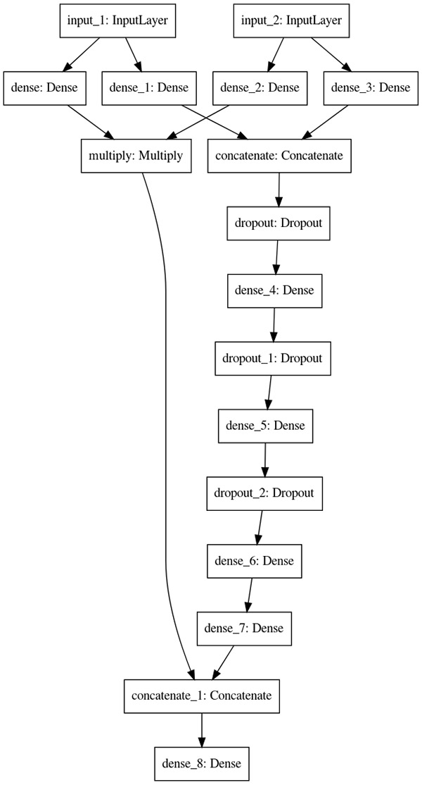
I use the Keras plot_model utility to verify the network architecture I just built is correct:

# build graph  
ncf_model = build_graph(n_user, n_item)  
  
# visualize and save to a local png file  
tf.keras.utils.plot_model(ncf_model, to_file="neural_collaborative_filtering_model.png")  

The output architecture should look like the following diagram.

Training and deploying the model

For instructions on deploying a model you trained using an instance on Amazon SageMaker, see Deploy trained Keras or TensorFlow models using Amazon SageMaker. For this post, I deploy this model using Script Mode.

We first need to create a Python script that contains the model training code. I compiled the model architecture code presented previously and added additional code required in the ncf.py, which you can use directly. I also implemented a function for you to load training data; to load testing data, the function is the same except the file name is changed to reflect the testing data destination. See the following code:

def _load_training_data(base_dir):  
    """ load training data """  
    df_train = np.load(os.path.join(base_dir, 'train.npy'))  
    user_train, item_train, y_train = np.split(np.transpose(df_train).flatten(), 3)  
    return user_train, item_train, y_train  

After downloading the training script and storing it in the same directory as the model training notebook, we can initialize a TensorFlow estimator with the following code:

ncf_estimator = TensorFlow(  
    entry_point='ncf.py',  
    role=role,  
    train_instance_count=1,  
    train_instance_type='ml.c5.2xlarge',  
    framework_version='2.1.0',  
    py_version='py3',  
    distributions={'parameter_server': {'enabled': True}},  
    hyperparameters={'epochs': 3, 'batch_size': 256, 'n_user': n_user, 'n_item': n_item}  
)  

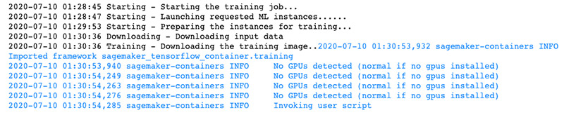
We fit the estimator to our training data to start the training job:

# specify the location of the training data  
training_data_uri = os.path.join(f's3://{bucket_name}', 'data')  
  
# kick off the training job  
ncf_estimator.fit(training_data_uri)  

When you see the output in the following screenshot, your model training job has started.

When the model training process is complete, we can deploy the model as an endpoint. See the following code:

endpoint_name = “neural-collaborative-filtering-model-demo”
model_name = “neural-collab-filtering-model”
predictor = ncf_estimator.deploy(
initial_instance_count=1,
      instance_type='ml.c5.xlarge',
endpoint_type='tensorflow-serving',
endpoint_name=endpoint_name,
model_name=model_name
)

Performing model inference

To make inference using the endpoint on the testing set, we can invoke the model in the same way by using TensorFlow Serving:

# Define a function to read testing data  
def _load_testing_data(base_dir):  
    """ load testing data """  
    df_test = np.load(os.path.join(base_dir, 'test.npy'))  
    user_test, item_test, y_test = np.split(np.transpose(df_test).flatten(), 3)  
    return user_test, item_test, y_test  
  
# read testing data from local  
user_test, item_test, test_labels = _load_testing_data('./ml-latest-small/s3/')  
  
# one-hot encode the testing data for model input  
with tf.compat.v1.Session() as tf_sess:  
    test_user_data = tf_sess.run(tf.one_hot(user_test, depth=n_user)).tolist()  
    test_item_data = tf_sess.run(tf.one_hot(item_test, depth=n_item)).tolist()  
      
# make batch prediction  
batch_size = 100  
y_pred = []  
for idx in range(0, len(test_user_data), batch_size):  
    # reformat test samples into tensorflow serving acceptable format  
    input_vals = {  
     "instances": [  
         {'input_1': u, 'input_2': i}   
         for (u, i) in zip(test_user_data[idx:idx+batch_size], test_item_data[idx:idx+batch_size])  
    ]}  
   
    # invoke model endpoint to make inference  
    pred = predictor.predict(input_vals)  
      
    # store predictions  
    y_pred.extend([i[0] for i in pred['predictions']])  

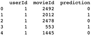
The model output is a set of probabilities, ranging from 0 to 1, for each user-item pair that we specify for inference. To make final binary predictions, such as like or not like, we need to apply a threshold. For demonstration purposes, I use 0.5 as a threshold; if the predicted probability is equal or greater than 0.5, we say the model predicts the user will like the item, and vice versa.

# combine user id, movie id, and prediction in one dataframe  
pred_df = pd.DataFrame([  
    user_test,  
    item_test,  
    (np.array(y_pred) >= 0.5).astype(int)],  
).T  
  
# assign column names to the dataframe  
pred_df.columns = ['userId', 'movieId', 'prediction']  

Finally, we can get a list of model predictions on whether a user will like a movie, as shown in the following screenshot.

Conclusion

Designing a recommender system can be a challenging task that sometimes requires model customization. In this post, I showed you how to implement, deploy, and invoke an NCF model from scratch in Amazon SageMaker. This work can serve as a foundation for you to start building more customized solutions with your own datasets.

For more information about using built-in Amazon SageMaker algorithms and Amazon Personalize to build recommender system solutions, see the following:

To further customize the Neural Collaborative Filtering network, Deep Matrix Factorization (Xue et al., 2017) model can be an option.


About the Authors

Ray Li is a Sr. Data Scientist with AWS Professional Services. His specialty focuses on building and operationalizing AI/ML solutions for customers of varying sizes, ranging from startups to enterprise organizations. Outside of work, Ray enjoys fitness and traveling.

Nick Biso is a Machine Learning Engineer at AWS Professional Services. He solves complex organizational and technical challenges using data science and engineering. In addition, he builds and deploys AI/ML models on the AWS cloud. His passion extends to his proclivity for travel and diverse cultural experiences.