How to store historical geospatial data in AWS for quick retrieval

One of the best examples of “big data” is weather data. Because weather data is geospatial and also has a time component, even working with a single measurement (such as temperature) over time and space can result in extraordinarily large sets of data.

For example, consider a raster dataset that contains temperature data, stored hourly for each location on an imaginary grid across the Earth that is 3600 units wide and 1801 units high. That’s over 150 million data points per day. A year’s worth of that data results in almost 57 billion data points. Datasets of that size are hard to move, hard to create, and hard to query efficiently.

That said, many workloads relating to weather data are analytic in nature and aren’t time critical. If you’re building a climate model, querying for the data to train it can take seconds or minutes, which generally isn’t a concern since the model training itself usually takes much longer–hours or even days. However, there are other workloads where query time is a more critical issue, such as when you’re building a user interface (UI) that needs to be responsive. In that example, you need a way to store weather data that can handle very large volumes of data while also supporting fast querying.

Amazon DynamoDB is the solution.

In this blog post, learn how to store historical geospatial data, such as weather data, on Amazon Web Services (AWS) using Amazon DynamoDB. This approach allows for virtually unlimited amounts of data storage combined with query performance fast enough to support an interactive UI. This approach can also filter by date or by location, and enables time- and cost- efficient querying.

How DynamoDB stores data

DynamoDB isn’t a relational database. Instead of rows and columns it has items and attributes, and tables aren’t joined together when querying. Instead, it’s a key-value data store, which means that for a given key, it can quickly store or retrieve a corresponding value. It’s virtually unlimited in terms of how much data it can store, and requires no maintenance since it’s a fully managed service.

To use DynamoDB effectively, there are a couple of important concepts to understand: key design and knowing how the data is organized into blocks (sometimes known as “chunks”).

First, every DynamoDB table must contain a primary key that uniquely identifies each item in the table. A DynamoDB primary key can have either one or two attributes, with one attribute defined as the partition key and, optionally, a second attribute defined as the sort key. The solution described in this blog post uses a primary key that contains both a partition key and a sort key (this is called a composite primary key).

DynamoDB combines these two parts when storing or retrieving data, and each plays a unique role. The partition key influences where data is physically stored, and the sort key can be used when selecting ranges of data.

When you run a query, DynamoDB first looks for items that contain an exact match of the partition key value you provide (equality is the only comparison operator supported for a partition key). Of those items with a matching partition key value, it then filters using the sort key value and comparison operator(s) you provide (sort keys support comparisons such as less-than, greater-than, or between).

The second important concept when working with DynamoDB is the idea that data is stored and retrieved in blocks that are 4K in length. That means if you’re retrieving data that’s 13,500 bytes long, DynamoDB actually retrieves 16,384 bytes spread across four blocks of 4K each. The speed and cost of a query depends on the number of blocks being returned. Therefore, it’s important to store data efficiently so you aren’t paying for retrievals of data that won’t be used.

Storing weather data in DynamoDB

This blog post walks through data retrieval considerations for an interactive UI that displays historical geospatial data based on select inputs—for example, a map-based interface that lets you select a location to get historical temperature data. The first step in designing how to efficiently store this data is to examine it thoroughly and think about how it will be used.

For this example, we work with historical weather data that’s available on the Registry of Open Data on AWS. The ERA5 dataset, published by the European Centre of Medium Range Forecasts (ECMWF), is known as a reanalysis dataset, which means that data points are a blend of observations and past short-range weather forecasts run with modern weather forecasting models. ERA5 contains measurements relating to temperature, wind speed and direction, dew point, and more, and data points are typically provided hourly for each point on a 1801×3600 grid, which is one-tenth of a degree of latitude or longitude.

Given that we know that all latitude values and longitude values are numbers with a single digit after the decimal point (e.g., 12.4), we can make some decisions about how best to store the data. First, we use the partition key to store the latitude and longitude. This is because a UI usually retrieves historical data for a given location rather than for a range of locations. Imagine a map-based interface, with which a user can select a location to get historical temperature data – that’s the type of use case we want to design for. Of course, a UI may be designed to retrieve data from multiple locations, and that can be handled by one query per location.

Further, when we retrieve historical data for a location, we probably want to filter the data by date. That means we want the option to select all data before a particular date, after a given date, or between two dates. For this UI use case, it’s probably reasonable to keep the granularity of the data to days or months rather than hours. Although we can filter data by hour once we retrieve the data from DynamoDB, generally, when we do a retrieval, it’s likely that we want at least one month’s worth of data. Also, storing a month’s worth of data at a time efficiently uses the 4K block size that DynamoDB uses.

Given these considerations, we can design our partition keys and design our sort keys for DynamoDB in the following manner:

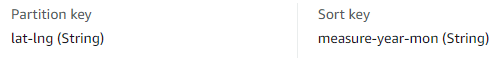
Figure 1. Illustration of names and types of partition and sort keys used in this approach, in which the partition key is noted as lat-lng (String) and the sort key as measure-year-mon (String).

Figure 1. Illustration of names and types of partition and sort keys used in this approach, in which the partition key is noted as lat-lng (String) and the sort key as measure-year-mon (String).

The partition key is a string that combines both the target latitude and longitude. For example, if we want to retrieve data for latitude 34.5 and longitude 229.6, the resulting partition key would be a string with the value “34.5-229.6” (concatenated with a hyphen between the values). Because different geospatial datasets use different indexing—latitudes and longitudes may be more or less granular than 0.1 degree—you can adjust this rounding as needed to suit your data.

The sort key combines the measurement type, the year, and the month into a single value. The ERA5 dataset contains one measurement per hour for a given variable, meaning that one 30-day month would contain 24 * 30 = 720 measurements. Instead of storing each of these 720 measurements separately, we store one month of data at a time in one DynamoDB item indexed by a single partition and sort key. Using this approach allows us to store more data per key than if we stored one day or even one hour at a time, which is more efficient in terms of storage costs and retrieval speed.

Why include the measurement name as part of the sort key? It allows us to use a single DynamoDB table for many different kinds of measurements. If you want to store temperature data and windspeed at 10 meters, you can use a letter to indicate the type of data, such as the letter “t” for temperatures, and “w” for windspeed. For example, if you are storing temperature data for December of 2019, then the resulting sort key would be a string with the value “t-2019-12.” Windspeed data for the same month would have a resulting sort key of “w-2019-12.”

Now that the keys have been designed, what about the values? The key structure we just defined means that each item in the DynamoDB table stores one month’s worth of data for a given measurement, at a given latitude/longitude. Assuming a 30-day month, a full month’s worth of data consists of 720 data points, which we store in a list.

This means that when you retrieve all the temperature data for a single month, you get a list of numeric values. The first item in the list is the temperature for the first hour of the first day of the month, the second item in the list is the temperature for the second hour of the first day of the month, and so forth. To put it another way, the first 24 values in the list are the measurements for the first day, the second 24 values in the list are the measurements for the second day, and the last 24 values in the list are the hourly temperatures for the thirtieth day.

Storing one month of data per DynamoDB item is also cost-effective. Since each data point in the ERA5 data set is a floating-point number (four bytes of storage used for each), the total size of the one month of data for one measurement, at one location, is 4 * 24 * 30 = 2880 bytes. Since this is less than DynamoDB’s 4K chunk size, a full month of data can be retrieved using one read request unit, which is how DynamoDB bills for reads.

Loading weather data into DynamoDB

Given this design, let’s discuss how to load the weather data into the DynamoDB table. One of the major issues that arises when dealing with big data such as weather data is the sheer volume of data. The ERA5 dataset has 1801 latitudes by 3600 longitudes by 24 values per day––all of which adds up to 156 million data points per day, per measurement. Ingesting a month’s worth of data for a single measurement therefore means handling roughly 4.6 billion data points.

Often, attempts to manipulate data of this size results in an out-of-memory exception or an out-of-disk-space exception. The only way to get around these restrictions is to isolate small pieces of the data and process those one at a time. We recommend selecting the data by one latitude at a time. This means collecting data for a single latitude value (such as 72.6) across all longitudes for a single metric like temperature. Once the data is collected, it can be stored in DynamoDB. Once one latitude has been processed and the resulting data has been stored in DynamoDB, you can move to the next latitude and repeat the process until all latitudes and longitudes have been processed. This approach reduces the amount of memory used because a smaller set of data is used at any given time.

Querying the DynamoDB table

There are two main ways to retrieve data from a DynamoDB table: querying and scanning. Querying is much faster and far more efficient than scanning, which looks at every row in the table. Querying is the recommended method to retrieve geospatial data from DynamoDB.

Querying requires the use of a partition key. As mentioned previously, you should use your existing knowledge about how the keys of the DynamoDB table are constructed when doing a query. That means adjusting a query latitude and longitude to correspond to partition key values used in the database. In a map-based UI, the latitude and longitude a user selects––for example, 41.8935 and 20.7653––would be rounded to one decimal place and concatenated with a hyphen. This rounding essentially “snaps” longitudes and latitudes to the nearest value that has data. When that’s done, the DynamoDB query can be performed with the partition key value set to the desired latitude/longitude combination.

Once the desired partition key is set, you also have the option to filter using the sort key and comparison operators. If you don’t specify a sort key, the query returns all data that matches the partition key, which is the latitude/longitude combination previously discussed. Note that when you specify only a partition key, you’ll get a huge amount of data returned for any variables stored in the table (temperature, wind speed, and whatever else you’ve ingested), for all the months and years that were stored. This isn’t generally desired behavior, so when querying we recommend you specify a sort key as well as a partition key.

In fact, you can specify a variety of conditions relating to the sort key. You can ask for all data greater than or equal to a sort key value (such as “t-2019-12”), all data less than or equal to a sort key, or all data that falls between two specified sort key values.

Measuring query performance

The following table shows DynamoDB query performance for a single measurement at a single location—that is, a single latitude/longitude combination—with a varying number of months:

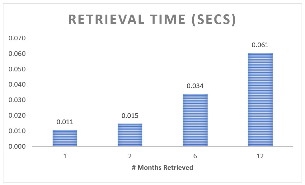
Figure 2. Chart showing query retrieval times for a single location with one, two, six, or 12 months of climate data.

Figure 2. Chart showing query retrieval times for a single location with one, two, six, or 12 months of climate data.

The chart shows that retrieval performance is roughly linear, based on the number of months retrieved. For example, using a sort key to retrieve 12 months of data takes slightly less than twice the time taken for six months.

Note that retrieving data for multiple latitude/longitude locations requires one query per location because each location has a unique partition key. This means that querying data for two locations takes twice as long as querying data for one location if we assume the number of months being retrieved is the same for each location.

Conclusion

Query time generally isn’t a concern when dealing with large amounts of weather data. Often, weather data—or any other large datasets of geospatial, historical data—is used to train climate models, and quick retrieval times aren’t as important as other factors. But there are occasions where speed is important, such as when you need to retrieve large amounts of data for a UI. For this example, DynamoDB is a good choice because it supports virtually unlimited amounts of data, and––when using well-designed keys––has extremely quick query times. Additionally, the use of a DynamoDB sort key allows filtering query results by measurement type and date. This flexibility allows sophisticated queries over time periods.

To read guidance about the effective designs of DynamoDB partition keys, refer to “Best practices for designing and using partition keys effectively.” For guidance about creating sort keys, refer to “Best practices for using sort keys to organize data.”

If you’re interested in using weather data on AWS for analytic purposes rather than interactively, please refer to the blog post “Decrease geospatial query latency from minutes to seconds using Zarr on Amazon S3,” which shows how to use tools such as Dask and Xarray to perform distributed queries of a central Amazon Simple Storage Service (Amazon S3) dataset.

Read related stories on the AWS Public Sector Blog:

Subscribe to the AWS Public Sector Blog newsletter to get the latest in AWS tools, solutions, and innovations from the public sector delivered to your inbox, or contact us.

Please take a few minutes to share insights regarding your experience with the AWS Public Sector Blog in this survey, and we’ll use feedback from the survey to create more content aligned with the preferences of our readers.