Creating satellite communications data analytics pipelines with AWS serverless technologies

Satellite communications (satcom) networks typically offer a rich set of performance metrics, such as signal-to-noise ratio (SNR) and bandwidth delivered by remote terminals on land, sea, or air. Customers can use performance metrics to detect network and terminal anomalies and identify trends to impact business outcomes, such as improving service level agreements (SLA). However, this is traditionally challenging due to issues like a lack of data science expertise, siloed data repositories, and high-cost business intelligence (BI) tools.

This walkthrough presents an approach using serverless resources from Amazon Web Services (AWS) to build satcom control plane analytics pipelines. Given bursts of time-series metrics, the presented architecture transforms the data to extract key performance indicators (KPIs) of interest. It then renders them in BI tools, such as displaying data-rate trends on a geo-map, and applies machine learning (ML) to flag unexpected SNR deviations.

The audience for this architecture is primarily satellite operators; however the presented serverless data analytics pipelines can be applied to a broader set of customers. This blog post demonstrates how to achieve business objectives with low/no-code analytics solutions, enabling new insights without the need for a plethora of data scientists. Plus, learn the benefits of using serverless solutions including automatic scaling, low costs, and reduced operational overheads.

Prerequisites

To create these AWS pipelines you must have an AWS account and a role with sufficient access to create resources in the following services:

Use cases for satellite communications data analytics pipelines

Satellite operators offer solutions for use cases ranging from Earth observation (EO) to satellite communications. In the latter scenario, a typical network layout ( Figure 1) involves communications from a remote terminal, such as a ship or aircraft equipped with a modem and antenna, through a satellite in a given orbit to a central gateway earth station called a teleport. At the teleport, the radio signal is down-converted to a lower intermediate frequency, and subsequently (de)modulated and (de)coded to extract or encode the payload. A network management system (NMS), often in a different location than the teleports, performs the orchestration function – for example commanding different quality of service (QoS) profiles depending on the type of user traffic.

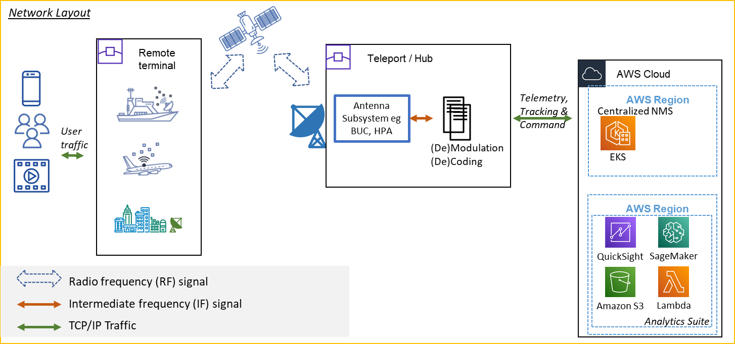
Figure 1. Network layout for a typical satellite communications service with analytics applied.

Throughout this architecture there are a variety of key metrics which are essential to monitor and act on if thresholds are breached to avoid SLA impact. A selection of these are:

Carrier-to-noise ratio (C/N): This is a measure of the received carrier strength relative to noise. Various factors such as weather, often termed as “rain fade,” can contribute to C/N.
Modulation and coding rates (MODCOD): This term covers converting data into RF for satellite antenna transmission, and the associated error correction typically via redundant bits. Popular satcom waveforms like DVB-S2X allow for modems to adapt dynamically to higher MODCOD rates, yielding more bits per Hertz and therefore greater throughput (i.e. higher efficiency) with the same bandwidth.
Receive lock lost: If the remote terminal is no longer able to receive or transmit the satellite because of issues like obstructions, the “lock” on the carrier signal may be lost, causing a discontinuity in user traffic.

Customers of satcom services might use such KPIs to determine efficiency and raise alarms if an unusual number of receive lock losses occur, or high packet-loss is measured.

Setting up AWS serverless data analytics pipelines

Now, let’s walk through how to set up a series of data analytics pipelines using AWS serverless best practices. We show how to use these services to reduce both cost and operational overhead, as these services only run when incoming data is being processed. The code and scripts for this tutorial are available at the AWS samples GitHub location under the satellite-comms-analytics-aws repository. You can use the AWS CloudFormation templates to provision any of these pipelines in your own AWS account, connecting your data sources to the entry point.

In this blog post, we explore the following use-cases:

Pipeline 1: Generating insights with a data lake, ETL transformation, and BI visualization tools
Pipeline 2: Visualizing real-time KPIs with Amazon OpenSearch Service
Pipeline 3: Detecting anomalies in SNR with machine learning

We start with the Amazon Kinesis Data Generator (KDG) which makes it simple to send randomized test data to either Amazon Kinesis Data Firehose or Amazon Kinesis Data Streams. Follow the steps in the KDG documentation to create an Amazon Cognito user with permissions to access Amazon Kinesis. You can then enter one of the sample record templates in the kdg/ folder, at which point the setup should match Figure 2 with the chosen AWS region, stream and satellite beam details.

Figure 2. Dataset representing satcom stream of key metrics.

Pipeline 1: Generating insights with a data lake, ETL transformation, and BI visualization tools

The first analytics use-case focuses on ingesting streaming data; performing extract, transform, and load (ETL) operations such as filtering or joining; then deriving business insights with analytics visualization tooling such as Amazon QuickSight.

Figure 3 presents a reference architecture that is the end result of running the streaming_s3_glue_pipeline.yaml template. This architecture includes an ETL job that created a structured dataset ready for viewing with Amazon QuickSight BI dashboards.

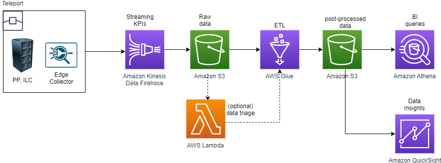
Figure 3. Streaming Kinesis Data Firehose pipeline with ETL transformation.

To deploy this solution in your own AWS account, select “Create stack (with new resources)” in the CloudFormation console. Next, download the streaming_s3_glue_pipeline.yaml template from the GitHub repository, select “Upload a template file” and browse to the yaml file.

After picking a stack name, supply some assets, such as Amazon S3 buckets, as parameters.

Figure 4. Satcom streaming pipeline CloudFormation template parameters.

Create three buckets in Amazon S3 – one for the KDG input data, one for the outputs of the AWS Glue ETL job, and one for the helper AWS Lambda and AWS Glue scripts. While this solution can be achieved with one bucket and sub-folders, the structure is intended to mimic a larger-scale data lake in which different functional groups may have access to some assets but not others.

Note: Supplying Amazon S3 input and output bucket names with no underscores or dashes enables downstream AWS Glue table automation without manual intervention.

The Lambda function which post-processes the Kinesis Data Firehose stream is supplied as Python source code in the GitHub repository. There are several ways to automate the deployment of Lambdas: one is to embed the code directly in the yaml file, another is to reference the code as a zip file in an Amazon S3 bucket. We use the latter mechanism. Simply zip up the Python function and add it to the SatComAssetsS3Bucket, similar to the KdfLambdaZipName parameter supplied previously.

You can now deploy the stack. Choose Next, acknowledge the IAM resources creation, and select Submit. It will take 5-10 minutes to complete the deployment of all AWS resources.

Generating sample Satcom data

In the KDG tool, select the newly created Kinesis Data Firehose stream, and select Send Data. After sending approximately 2,000 records, select Stop. You can check that the Lambda transformation function triggered by observing the /aws/lambda/function-name Log Group in Amazon CloudWatch. The resultant JSON objects will be available in your InputS3Bucket.

Figure 5. JSON objects in the Amazon S3 input bucket produced by KDG.

Creating AWS Glue Catalog and ETL transformation

We use AWS Glue in this pipeline for several reasons. First, it helps support schema discovery establishing which fields we want to keep or modify. Second, it generates a structured, partitioned data catalog we can efficiently query. Third, it allows transformations so we can apply any filtering or joining of the dataset.

The CloudFormation template generates AWS Glue Data Catalog databases for input and output results, a crawler for schema discovery, and a job to transform the JSON records.

The first step is to run the AWS Glue crawler. We only need to run this once since our KDG sample data format does not change. The crawler takes about a minute to run and generates one table with Apache Hive style year/month/day/hour partitions.

Next, find the generated AWS Glue job via the AWS console, under Jobs. This job originated as a visual workflow in AWS Glue Studio which makes it simple to string multiple transformations together. Once complete, the script was modified to parameterize the database and table entries, enabling the PySpark job to be re-used in automated pipelines.

The actual transformation in this job is simple – a Python regular expression matching remote terminals beginning with “C”:

Filter_node1670204808887 = Filter.apply(
    frame=ApplyMapping_node2,
    f=lambda row: (bool(re.match("^C", row["remoteid"]))),
    transformation_ctx="Filter_node1670204808887",
)

Select Run to start the AWS Glue job – it should complete in 1-2 minutes, delivering transformed JSON objects to the output Amazon S3 Bucket.

Obtaining data insights with Amazon Athena

The process of AWS Glue cataloging automatically creates tables that can be queried in Athena. Open the Athena console and select the AWS Glue Catalog results database. Select the three dots to the right of the table and choose Preview Table. It will generate a query similar to the following:

SELECT * FROM "satcom-glue-cat-db-results"."satcomkdfbucketresults" limit 10;

Run the query and observe the resulting metrics.

Troubleshooting tip: If you find that Athena is not returning the most recent results, it may be that the new partitions are not being picked up. Simply run the following in Athena to add new partitions:

MSCK REPAIR TABLE satcomkdfbucket

Visualizing key business insights in Amazon QuickSight

Open Amazon QuickSight and select Datasets. QuickSight can ingest data from a wide range of AWS services such as Amazon S3, Amazon Relational Database Service (Amazon RDS), and also various third-party tools. Select Athena as the data source. Give the table a name, then select the resulting database and table.

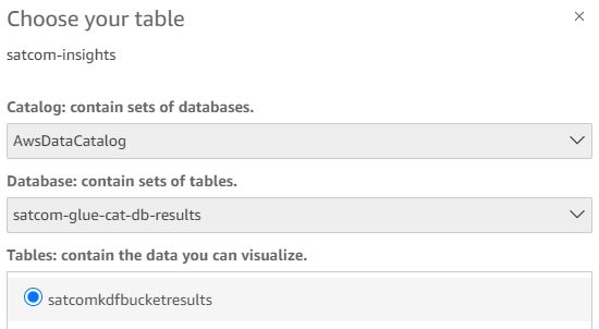
Figure 6. Amazon QuickSight dataset selection.

Generating feature-rich analyses and dashboards is then a matter of dragging and dropping visualizations in QuickSight. Note that for mobile endpoints, the geospatial visualization is particularly useful since we can plot metrics by latitude and longitude on a map.

Figure 7. Amazon QuickSight dashboard of key satcom metrics.

One final observation regarding the dashboard is that the insight at the bottom-right is a machine learning-based insight. No complex data science background is required; QuickSight simply generates ML observations such as anomaly detection based on the datasets presented.

In completing Pipeline 1, we created a visual overview of key satcom metrics; a structured, scalable data lake that enables fast querying; the capability to run jobs as needed without standing up permanent compute instances; and the ability to find anomalies without specialized ML data science knowledge.

With this pipeline, satcom operators can identify revenue-impacting KPI trends quicker and act on anomaly alerts.

Pipeline 2: Real-time monitoring in Amazon OpenSearch Service

What if we need to observe certain KPIs in real-time, such as for a VIP flight or cruise ship?

Figure 8 represents a reference architecture for real-time streaming of metrics to Amazon OpenSearch Service, an open source, distributed search and analytics suite. Widgets such as heat-maps and geo-mapping can be added with ease to rapidly create rich BI dashboards.

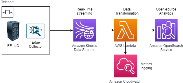
Figure 8. Real-time streaming to OpenSearch Service with inline data transformation.

The pipeline begins with Kinesis Data Streams. One of the key differences between Kinesis Data Streams and the Kinesis Data Firehose used in Pipeline 1 is that Kinesis Data Streams is intended for real-time data analytics, while Kinesis Data Firehose makes more sense for data lake use cases that use both current and historical data.

Kinesis Data Streams does however accommodate low-latency inline transformations via Lambda functions. The Python boto3 record processing required in this pipeline maps latitude and longitude coordinates to a geo_point OpenSearch Service field type.

    # create geo_point field from location dictionary with lat, long
    body = {
        "mappings": {
            "properties": {
                "location": {
                    "type": "geo_point"
                }
            }
        }
    }
    try:
        response = client.indices.create(index, body=body)
        print("Client index create response: ", response)
    except:
        print("Already created index: ", index)

Satcom operators can use the resulting index to plot a coordinate map. Operators can use the metric range color coding to monitor and take rapid action if a KPI is beyond a threshold or occurs at an unexpected geo-location.

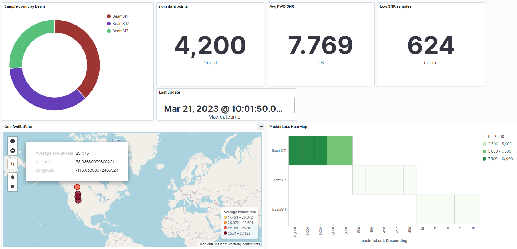
Figure 9. OpenSearch Service real-time dashboard with satcom KPIs.

Find the step by step instructions for how to create this dashboard in the README in the GitHub repository, under Analytics Pipelines.

Pipeline 3: Detecting anomalies in SNR with machine learning

Pipeline 3 uses the Amazon SageMaker Random Cut Forest algorithm to detect anomalous SNR values within the dataset generated in Pipeline 1. The algorithm can be implemented using either SageMaker or Amazon Kinesis Data Analytics. This walkthrough uses SageMaker, as this approach allows for greater control on specifying training data. The algorithm is deployed to a SageMaker Serverless Inference endpoint. The detected SNR value anomalies are written to an Amazon S3 bucket. Figure 10 represents the reference architecture defined in this pipeline.

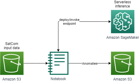
Figure 10. Pipeline 3 architecture which uses the SageMaker Random Cut Forest model to detect anomalies.

The detected anomalies are written to Amazon S3 in JSON lines format as seen in Figure 11. Amazon S3 Event Notifications can be configured so that downstream applications or alerts can be launched when the anomalies are written to Amazon S3.

Find the step-by-step instructions for Pipeline 3 in the README in the GitHub repository, under Analytics Pipelines.

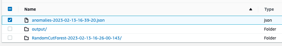
Figure 11. Write anomalies to Amazon S3.

This pipeline provides satcom operators with a machine learning model that can detect anomalies in the SNR or any other critical metric.

Solution costs

The final step in our satcom analytics journey is to outline the cost of the solutions.

As part of the Operational Excellence Pillar of the AWS Well-Architected Framework, we tag each of the resources via a consistent Name-Value schema. This allows us to create granular cost reports via AWS Cost Explorer.

Figure 12. Consistent name value tagging strategy for resources.

At the time of publication, if we cost out a realistic scenario and run the pipelines on an hourly basis, the total for all three pipelines comes to about the cost of a latte. The serverless nature of these services is the major reason for keeping the solutions low-cost, as they only run when the pipelines are invoked. At all other times, they do not incur any cost.

The major contributor to the cost is hosting the OpenSearch Service domain for Pipeline 2. However, as of January 2023, Amazon OpenSearch Serverless is now generally available. The net result is lower costs since you avoid potential over-provisioning and only pay for the compute and storage resources consumed.

AWS Lambda processing costs may be incurred if there are thousands of data ingest sites (teleports) or the code duration increases. Amazon QuickSight pricing is on a per-reader activity basis.

Conclusion

This walkthrough explores how to leverage AWS serverless analytics pipelines to derive valuable business insights in satcom use-cases. Operational teams can quickly see the effects of, for example, weather patterns at remote terminals or teleports via rich analytics dashboards. New machine learning models can detect anomalies and identify gaps in expected versus measured performance. Operators can measure enhanced business through SLA improvement.

Get started with the code repository to develop new analytics pipelines using the supplied CloudFormation templates as a baseline for your next workload.

For more aerospace and satellite learning resources, visit the AWS for Aerospace and Satellite main page.