Building a Data Processing and Training Pipeline with Amazon SageMaker

By Cesar Del Solar, Sr. Software Architect at Next Caller

Amazon SageMaker is a fully-managed machine (ML) learning service offered by Amazon Web Services (AWS), providing every developer and data scientist with the ability to build, train, and deploy ML models quickly.

At Next Caller, an AWS Partner Network (APN) Technology Partner, we have found Amazon SageMaker invaluable for driving our data analysis and processing pipeline.

In this post, I will walk through various features of Amazon SageMaker and the AWS ecosystem to show how we process and analyze hundreds of gigabytes of call metadata for Fortune 500 financial institutions and telecommunications providers through our primary service, VeriCall.

VeriCall verifies that a phone call is coming from the physical device that owns the phone number, and flags spoofed calls and other suspicious interactions in real-time.

This capability allows our clients to trust phone calls from legitimate customers while also creating an early opportunity to increase security for untrustworthy calls to stop phone fraud before it starts.

We use machine learning to understand call pathways through the telephone network, rendering analysis in approximately 125 milliseconds with our VeriCall analysis engine.

Next Caller tracks this metric using Amazon CloudWatch, and monitor it closely to ensure changes to our analyzer do not negatively impact this latency.

VeriCall Architecture

The diagram below is a top-down, simplified version of Next Caller’s API architecture. Phone call metadata from our customers comes in via API to VeriCall, which is implemented inside an AWS Lambda function.

The function encapsulates a small Pyramid web app with several endpoints, and is terminated by an Amazon API Gateway entry point. Our customers send data as JSON; we accept both dictionaries of SIP (Session Initiation Protocol) headers, or the raw base64-encoded SIP invite.

Depending on our customers’ integration needs, they can hit one of several endpoints; the standard one returns a score immediately, whereas a second endpoint will return a tracking ID. This tracking ID can be used in a subsequent request to return a risk score.

The Lambda function makes an API call to an Amazon SageMaker inference endpoint, running our custom Go-based inference code (more on that later). Once the inference comes back, Next Caller’s analysis code runs it through our rule engine and outputs a fraud/risk score back to the customer.

This entire loop must run as fast as possible, and we have found that Amazon SageMaker provides great performance and takes about 125 milliseconds on average for our current models.

Figure 1 – VeriCall architecture on AWS.

Customer data is also saved into Amazon Simple Storage Service (Amazon S3) via Amazon Simple Queue Service (SQS), a fully-managed message queuing service that enables you to decouple and scale microservices, distributed systems, and serverless applications.

Our data team of analysts and data scientists then use Amazon Athena to create queries on this data for further analysis inside an Amazon SageMaker notebook.

Using Amazon SageMaker Notebook for Analysis

At its core, Amazon SageMaker Notebook is a Jupyter notebook that adds a few features, such as direct integration with Git so that individual notebooks can be easily version-controlled, and the ability to quickly spin up an instance on various architectures, including multi-GPU instances.

Next Caller uses typical analysis tools such as Pandas and Matplotlib for the majority of our data work.

One great feature of Jupyter is the ability to add interactivity to your notebook with the ipywidgets library. For our analysts and data scientists to work with ML models, we built a simple ipywidgets-based user interface (UI) that interacts directly with the Amazon SageMaker Training API and Amazon Athena API to create queries and train on the resultant data.

Figure 2 – Our ipywidgets-based interface for interfacing with Amazon SageMaker training jobs.

As shown in the Query Parameters tab above, we built a simple interface to allow the user (one of our data analysts) to make an Amazon Athena query. They can add or remove datasets from the query, and set the number of data points from each dataset. In our case, these data points are calls and their metadata.

The Training Parameters tab allows users to set the various hyperparameters for the training job, such as number of epochs, learning rate, optimizer, etc.

Clicking the Start button creates an Amazon SageMaker training job with the resultant query data and hyperparameters.

One thing to note about Amazon SageMaker training jobs is they do not accept environment variables. Instead, we passed in anything that could be an environment variable as a hyperparameter instead.

In our training code, we handle these environment variables differently from regular hyperparameters, which we prefix with a string model. We then pass in the AWS CloudFormation stack name and region name as hyperparameters, in order for the training job to communicate its real-time status to an Amazon EventBridge pipeline.

Amazon EventBridge is a serverless event bus that makes it easy to connect applications together using data from your own applications, software-as-a-service (SaaS) applications, and AWS services.

Figure 3 – ipywidgets-based interface for visualizing training job results.

Another Jupyter interface was built for quickly visualizing model training statistics. In the image above, we used the Amazon S3 API to list the training jobs in a specific bucket, and clicking Display fetches the training stats, such as training and validation loss and accuracy, from an Amazon DynamoDB table.

The DynamoDB table is automatically updated during training with the help of a Lambda function that listens for Amazon EventBridge events that get emitted after every epoch.

When using Jupyter and the Amazon SageMaker Notebook, we can attach lifecycle configuration scripts to notebooks that run when these first boot up. In these scripts, we can install whichever requirements we like, or do any other initial setup.

By default, ipywidgets does not play nicely with Amazon SageMaker’s version of JupyterLab, so we had to add the following to the “Start Notebook” script:

# Add node to system path.
PATH=/home/ec2-user/anaconda3/envs/JupyterSystemEnv/bin/:$PATH
npm install -g ssh://git-codecommit.us-east-1.amazonaws.com/v1/repos/yarn echo 'yarn-path
"/home/ec2-user/anaconda3/envs/JupyterSystemEnv/lib/node_modules/yarn/bin/yarn.js"' > /home/ec2-user/anaconda3/envs/JupyterSystemEnv/lib/python3.6/site-packages/jupyterlab/staging/ .yarnrc
/home/ec2-user/anaconda3/envs/JupyterSystemEnv/bin/jupyter labextension install @jupyter-widgets/jupyterlab-manager

This script installs the newest version of the jupyter-widgets extension for JupyterLab, thus allowing us to use our ipywidgets interface in JupyterLab.

Amazon SageMaker Training Jobs and Using the GPU

In many cases, GPU training is more cost-effective than regular CPU training, and both are available on Amazon SageMaker. Some types of models parallelize particularly well, specifically those with multiple largely independent operations; for example, those that use convolutional neural networks (CNNs).

Even with non-CNN models, however, one can usually find a moderate speed boost when using GPUs for training.

Next Caller uses Keras with Tensorflow and Python 3 for training. Since we use our own training algorithms, we had to build a Docker image with a train executable. We use AWS CodeBuild to create this Docker image, and in the buildspec.yml file it’s important to log in to a hard-coded Amazon Elastic Container Registry (ECR) repository as follows:

$(aws ecr get-login --no-include-email --registry-ids 520713654638)

This repository contains the base Amazon SageMaker-compatible GPU training image. Our base Dockerfile then imports this image in its first line:

FROM 520713654638.dkr.ecr.us-east-1.amazonaws.com/sagemaker-tensorflow-scriptmode:1.12.0-gpu-py3

If you prefer to inherit from the base CPU image, just replace the gpu in the Docker image tag with cpu. This may be helpful for running tests during your build, particularly because AWS CodeBuild does not support GPU instances as of yet.

One more thing we learned the hard way, although we did find documentation for it after the fact, is to make sure you don’t overwrite the LD_LIBRARY_PATH in your Dockerfile. Everything will be linked properly if you don’t specify it at all; as the documentation states, you do not need to bundle the NVIDIA drivers with the image.

Overall, we increased our cost efficiency by about a factor of seven by switching to GPU instances. Although training time only decreased a bit, we were able to train on less costly instances. Your mileage may vary depending on the type of model you are training with.

Amazon SageMaker Inferences and Using the Go Language

At Next Caller, we are big fans of the Go programming language. It’s particularly suited to highly concurrent and low overhead APIs, but we also suspected it might improve the performance of our model inferences.

Our model inference code was originally written in Python 3 and suffered from a few issues, such as large memory usage, lack of concurrency in the web server, and occasional spikes in latency. Particularly, the P99 of inference latency was sometimes more than one or two seconds, which was unacceptable as this is part of an API with sub-200-millisecond latency.

Occasionally, requests would even time out. Using the Go language, we can instantiate just a small number of models in memory, build our own router with simple channels and goroutines, and avoid the relatively heavy threads and complexity of a Python + gunicorn + nginx stack.

We explored the Go Tensorflow library and found it was relatively easy to use. The more complex part is translating our Keras models to make them capable of using the raw Tensorflow integration, and updating our training code to save future models in such a way that they’re compatible with our new Go-based inference server.

The following Python code is a simplified version of what is needed to save a model to make it compatible with Go:

from keras import backend as K
import tensorflow

sess = tensorflow.Session()
sess.run(tensorflow.global_variables_initializer())
K.set_session(sess)
# instantiate and train your model, e.g.
model.fit(...)
builder = tensorflow.saved_model.builder.SavedModelBuilder('/path/')
builder.add_meta_graph_and_variables(sess, [f'tag_{pawn_name}'])
builder.save()

Note that you must provide a “tag” for each of your models, in order to load these later. In Go, you can then load the model as follows:

model, err := tf.LoadSavedModel(modelLocation, []string{"tag_" + modelName}, nil)

The tag should be the same tag used in the code that saves the model, and the modelLocation is just the path where the model was saved to. Your code can then invoke the particular model with an input vector as follows:

func (w *worker) invokeModel(input []float32) []float32 {
	tensor, _ := tf.NewTensor([][]float32{input})
	// Now run the prediction
	result, _ := w.model.Session.Run(
		map[tf.Output]*tf.Tensor{
			model.Graph.Operation(w.meta.inputLayerName).Output(0): tensor,
		},
		[]tf.Output{
			model.Graph.Operation(w.meta.inferenceLayerName).Output(0),
		},
		nil,
	)
	data := result[0].Value().([][]float32)
	return data[0]
}

Of course, you should be checking for errors instead of ignoring them, but the code is for demonstrating a simple inference.

Switching to Go for our inference code drastically decreased our P99 latency, from two seconds to just a couple hundred milliseconds, while CPU and memory usage either stayed the same or modestly decreased.

A/B Splitting and Auto Scaling

Amazon SageMaker allows you to split traffic between two different versions of a model, and we use this capability often. As the phone networks evolve and change, our models must keep up to date, and we train and deploy new versions of our models regularly.

As an additional layer of security, to ensure there’s no drastic changes in our scoring statistics, we deploy the new model to 10 percent of our traffic at first.

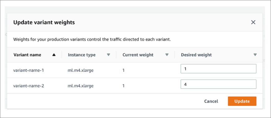
Figure 4 – Modifying model variant weights via Amazon SageMaker interface.

In the image above, we show how to create multiple model “variants” and a split for them. In this example, 80 percent of traffic would go to variant-name-2 and 20 percent to variant-name-1. This UI is available under the Amazon SageMaker Inference Endpoints settings.

We can then remove the old model entirely. Note that you can’t do a 100-0 split in the UI above. It would not be desirable because we’d have a set of idle variant instances with no traffic but accumulating charges. Rather, we remove them via a CloudFormation template change.

Amazon SageMaker also allows auto scaling your inference instances. As traffic ebbs and flows throughout the day, more instances can be deployed, depending on a chosen scaling policy.

For example, you can choose to deploy an additional instance if your number of inferences per second hits a certain threshold. The instances would then be deregistered automatically after your traffic dies down for a while. The interface shown below is also available under the Amazon SageMaker Endpoints panel.

Figure 5 – Setting up automatic scaling of Amazon SageMaker endpoints.

The Data Pipeline and Quality Assurance

We care very much about the quality of our data and do our best to ensure no fraudulent phone calls are getting marked as green in our system. We do this while still keeping the overall number of false positives (reds that are not actually fraud) as low as possible.

As such, whenever we train a new model, we use a semi-automatic approach to validate the model with our current VeriCall rule engine and a randomly chosen set of recent phone calls.

In order to run our inference code, we make the inference Docker image available to a data pipeline executable. The inference image can read lines from stdin and output inferences to stdout, where it can then be picked up by the next step in the pipeline.

Roughly, we use an approach like the following for our data pipeline:

cat to_analyze.csv | csv_to_json | append_model_request | docker run --rm -i {model_infer_docker_image} | analyze

There are a few key points here. First, the line above is meant to be run on Linux and uses pipes to pass data through from left to right. We start with a CSV file with call data; converting the CSV file to JSON lines (JSONL) makes our pipeline more readily parallelizable and scalable, despite the larger file size.

We don’t have to worry about the distinction between the CSV header and the rest of the data. Our csv_to_json program takes care of this conversion.

Next, append_model_request is an executable that appends a special key to each incoming JSON object with instructions for the inference image. The inference image is run directly with a docker run -i command, which allows it to connect directly to stdin and stdout.

As JSON lines come in, the inference image makes a prediction and outputs it directly to stdout for the final step: analyze.

This program is an interface into our VeriCall analysis engine, and takes in the model predictions along with the other parts of the call metadata to create a final score for a call.

The analysts can run this pipeline script directly as above, or through a simple wrapper script. In either case, the result can be piped directly to a file and further analyzed with Amazon SageMaker Notebook.

As we are typically testing hundreds of thousands to millions of calls at a time, we run this quality assurance (QA) process inside the notebook as well for greater efficiency. The other executables have been written to be multi-threaded so we can take advantage of the large, multi-CPU Amazon SageMaker instances.

Depending on the results of this QA process, the models and rules are further refined or finalized and made ready for the next deploy.

Tying Everything Together with AWS CloudFormation

The large majority of this stack is automatically set up via CloudFormation templates. We’re big believers in infrastructure-as-code, and setting it up this way allows for easily auditable and reproducible builds, despite some initial work setting these up.

As an example, we walk through setting up a model with two variants, along with an endpoint.

Model:
    Type: AWS::SageMaker::Model
    Properties:
      PrimaryContainer:
        Image: !Ref InferenceImageVersion
        ModelDataUrl: !Ref PrimaryModelDataUrl
        Environment:
          LOG_LEVEL: !Ref LogLevel
      ExecutionRoleArn: !GetAtt SageMakerExecutionRole.Arn

  SecondaryModel:
    Type: AWS::SageMaker::Model
    Properties:
      PrimaryContainer:
        Image: !Ref InferenceImageVersion
        ModelDataUrl: !Ref SecondaryModelDataUrl
        Environment:
          LOG_LEVEL: !Ref LogLevel
      ExecutionRoleArn: !GetAtt SageMakerExecutionRole.Arn

In the example above, we set up two models: a primary and a secondary model. Each uses the same InferenceImageVersion, which is a full ECR repository name and tag.

The ModelDataUrl for each model points to an S3 bucket containing the model tarballs. There’s also a SageMakerExecutionRole defined in the CloudFormation template, with a ManagedPolicyArn of arn:aws:iam::aws:policy/AmazonSageMakerFullAccess.

You can then define an EndpointConfig as follows:

EndpointConfig:
    Type: AWS::SageMaker::EndpointConfig
    Properties:
      ProductionVariants:
        - InitialInstanceCount: !Ref InstanceCount
          InitialVariantWeight: 9.0
          InstanceType: !Ref InstanceType
          ModelName: !GetAtt Model.ModelName
          VariantName: !GetAtt Model.ModelName

        - InitialInstanceCount: !Ref InstanceCount
          InitialVariantWeight: 1.0
          InstanceType: !Ref InstanceType
          ModelName: !GetAtt SecondaryModel.ModelName
          VariantName: !GetAtt SecondaryModel.ModelName

In this Endpoint Configuration, the weights are set at a nine-to-one split. You can modify these via the Amazon SageMaker user interface later, or via this template.

Finally, an Endpoint can be defined which uses this Endpoint Configuration:

Endpoint:
    Type: AWS::SageMaker::Endpoint
    Properties:
      EndpointConfigName: !GetAtt EndpointConfig.EndpointConfigName
      EndpointName: !Sub "${AWS::StackName}-pawn-endpoint"

About the only manual tasks we do is setting up a couple of the initial AWS Identity and Access Management (IAM) roles, and the Amazon SageMaker Notebook lifecycle configuration scripts.

Summary

In this post, we have shown how Amazon SageMaker has helped in our efforts to analyze large amounts of data, train and deploy machine learning models, and verify and further refine the performance of these models.

We used a number of varied AWS services for all the steps of this pipeline, especially leveraging the many functions of Amazon SageMaker, to take us from data analysis to production model deployment.

In addition, we used some newer services like Amazon EventBridge to allow us to more closely monitor the training in real-time, and tied it all together with AWS CloudFormation.

This solution can be easily scaled to handle many more requests by using Amazon SageMaker’s built-in auto scaling functionality and the inherent scalability of AWS Lambda and Amazon API Gateway.

The content and opinions in this blog are those of the third party author and AWS is not responsible for the content or accuracy of this post.

.

.

Next Caller – APN Partner Spotlight

Next Caller is an APN Advanced Technology Partner. Its technology verifies the call is coming from the physical device that owns the number, and uses machine learning and understanding of call pathways through the telephone network to render analysis quickly.

Contact Next Caller | Solution Overview

*Already worked with Next Caller? Rate this Partner

*To review an APN Partner, you must be an AWS customer that has worked with them directly on a project.