Build multi-class classification models with Amazon Redshift ML

November 2022: Post was reviewed and updated to announce support of Prediction Probabilities for Classification problems  using Amazon Redshift ML.

Amazon Redshift ML simplifies the use of machine learning (ML) by using simple SQL statements to create and train ML models from data in Amazon Redshift. You can use Amazon Redshift ML to solve binary classification, multi-class classification, and regression problems and can use either AutoML or XGBoost directly.

This post is part of a series that describes the use of Amazon Redshift ML. For more information about building regression using Amazon Redshift ML, see Build regression models with Amazon Redshift ML.

You can use Amazon Redshift ML to automate data preparation, pre-processing, and selection of problem type as depicted in this blog post. We assume that you have a good understanding of your data and what problem type is most applicable for your use case. This post specifically focuses on creating models in Amazon Redshift using the multi-class classification problem type, which consists on classifying instances into one of three or more classes. For example, you can predict whether a transaction is fraudulent, failed or successful, whether a customer will remain active for 3 months, six months, nine months, 12 months, or whether a news is tagged as sports, world news, business.

Prerequisites

To get started, we need an Amazon Redshift cluster or an Amazon Redshift Serverless endpoint and an AWS Identity and Access Management (IAM) role attached that provides access to SageMaker and permissions to an Amazon Simple Storage Service (Amazon S3) bucket.

For an introduction to Redshift ML and instructions on setting it up, see Create, train, and deploy machine learning models in Amazon Redshift using SQL with Amazon Redshift ML.

To create a simple cluster with a default IAM role, see Use the default IAM role in Amazon Redshift to simplify accessing other AWS services.

Use case

For our use case, we want to target our most active customers for a special customer loyalty program. We use Amazon Redshift ML and multi-class classification to predict how many months a customer will be active over a 13-month period. This translates into up to 13 possible classes, which makes this a better fit for multi-class classification. Customers with predicted activity of 7 months or greater are targeted for a special customer loyalty program.

Input raw data

To prepare the raw data for this model, we populated the table ecommerce_sales in Amazon Redshift using the public data set E-Commerce Sales Forecast, which includes sales data of an online UK retailer.

Enter the following statements to load the data to Amazon Redshift:

Alternately we have provided a notebook you may use to execute all the sql commands that can be downloaded here. You will find instructions in this blog on how to import and use notebooks.

CREATE TABLE IF NOT EXISTS ecommerce_sales
(
	invoiceno VARCHAR(30)   
	,stockcode VARCHAR(30)   
	,description VARCHAR(60)    
	,quantity DOUBLE PRECISION   
	,invoicedate VARCHAR(30)    
	,unitprice    DOUBLE PRECISION
	,customerid BIGINT    
	,country VARCHAR(25)    
)
;

Copy ecommerce_sales
From 's3://redshift-ml-multiclass/ecommerce_data.txt'
iam_role default delimiter '\t' IGNOREHEADER 1 region 'us-east-1' maxerror 100;

Data preparation for the ML model

Now that our data set is loaded, we can optionally split the data into three sets for training (80%), validation (10%), and prediction (10%). Note that Amazon Redshift ML Autopilot will automatically split the data into training and validation, but by splitting it here, you will be able to verify the accuracy of your model. Additionally, we calculate the number of months a customer has been active, as it will be the value we want our model to predict on new data. We use the random function in our SQL statements to split the data. See the following code:

create table ecommerce_sales_data as (
  select
    t1.stockcode,
    t1.description,
    t1.invoicedate,
    t1.customerid,
    t1.country,
    t1.sales_amt,
    cast(random() * 100 as int) as data_group_id
  from
    (
      select
        stockcode,
        description,
        invoicedate,
        customerid,
        country,
        sum(quantity * unitprice) as sales_amt
      from
        ecommerce_sales
      group by
        1,
        2,
        3,
        4,
        5
    ) t1
);

Training Set

create table ecommerce_sales_training as (
  select
    a.customerid,
    a.country,
    a.stockcode,
    a.description,
    a.invoicedate,
    a.sales_amt,
    (b.nbr_months_active) as nbr_months_active
  from
    ecommerce_sales_data a
    inner join (
      select
        customerid,
        count(
          distinct(
            DATE_PART(y, cast(invoicedate as date)) || '-' || LPAD(
              DATE_PART(mon, cast(invoicedate as date)),
              2,
              '00'
            )
          )
        ) as nbr_months_active
      from
        ecommerce_sales_data
      group by
        1
    ) b on a.customerid = b.customerid
  where
    a.data_group_id < 80
);

Validation Set

create table ecommerce_sales_validation as (
  select
    a.customerid,
    a.country,
    a.stockcode,
    a.description,
    a.invoicedate,
    a.sales_amt,
    (b.nbr_months_active) as nbr_months_active
  from
    ecommerce_sales_data a
    inner join (
      select
        customerid,
        count(
          distinct(
            DATE_PART(y, cast(invoicedate as date)) || '-' || LPAD(
              DATE_PART(mon, cast(invoicedate as date)),
              2,
              '00'
            )
          )
        ) as nbr_months_active
      from
        ecommerce_sales_data
      group by
        1
    ) b on a.customerid = b.customerid
  where
    a.data_group_id between 80
    and 90
);

Prediction Set

create table ecommerce_sales_prediction as (
  select
    customerid,
    country,
    stockcode,
    description,
    invoicedate,
    sales_amt
  from
    ecommerce_sales_data
  where
    data_group_id > 90);

Create the model in Amazon Redshift

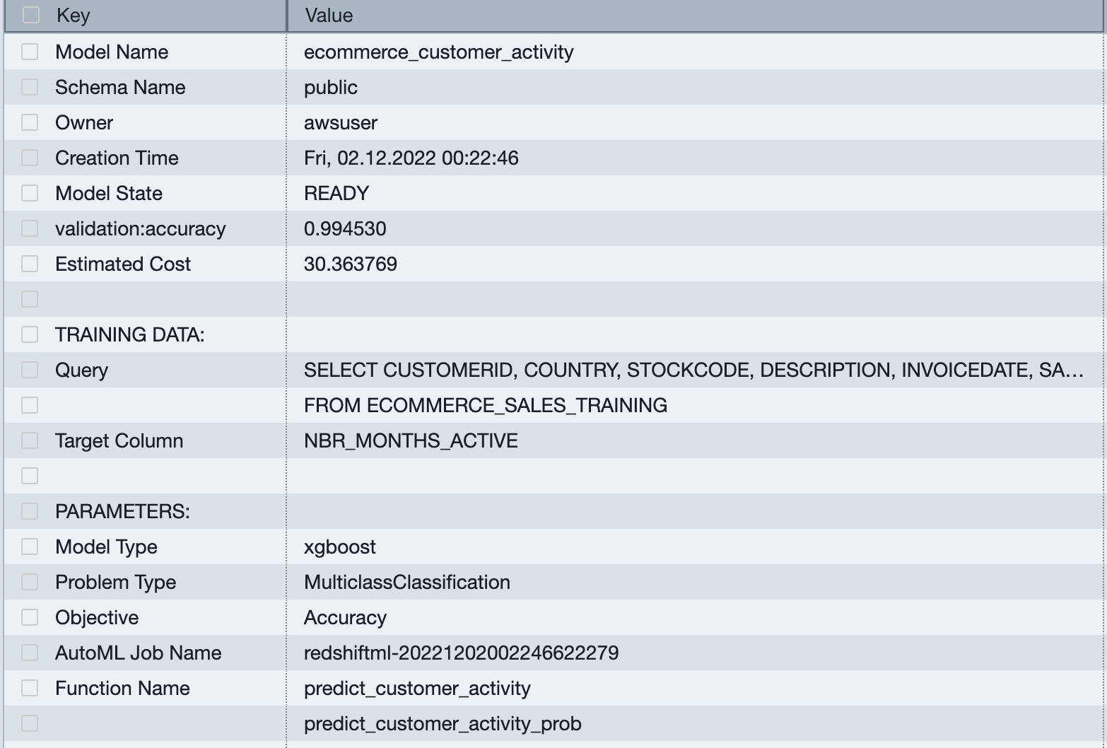
Now that we created our training and validation data sets, we can use the create model statement in Amazon Redshift to create our ML model using Multiclass_Classification. We specify the problem type but we let AutoML take care of everything else. In this model, the target we want to predict is nbr_months_active. Amazon SageMaker creates the function predict_customer_activity, which we use to do inference in Amazon Redshift. See the following code:

create model ecommerce_customer_activity
from
  (
Select
  Customerid,   
  country,
  stockcode,
  description,
  invoicedate,
  sales_amt,
  nbr_months_active  
 from ecommerce_sales_training)
 TARGET nbr_months_active FUNCTION predict_customer_activity
 IAM_ROLE default
 problem_type MULTICLASS_CLASSIFICATION  
  SETTINGS (
    S3_BUCKET '<<your-amazon-s3-bucket>>',
    S3_GARBAGE_COLLECT OFF,
    MAX_RUNTIME 9600
    
  );

Validate predictions

In this step, we evaluate the accuracy of our ML model against our validation data.

While creating the model, Amazon SageMaker Autopilot automatically splits the input data into train and validation sets, and selects the model with the best objective metric, which is deployed in the Amazon Redshift cluster. You can use the show model statement in your cluster to view various metrics, including the accuracy score. If you don’t specify explicitly, SageMaker automatically uses accuracy for the objective type. See the following code:

Show model ecommerce_customer_activity;

As shown in following output, our model has an accuracy score of 0.994530.

Let’s run inference queries against our validation data using the following SQL code against the validation data:

select 
 cast(sum(t1.match)as decimal(7,2)) as predicted_matches
,cast(sum(t1.nonmatch) as decimal(7,2)) as predicted_non_matches
,cast(sum(t1.match + t1.nonmatch) as decimal(7,2))  as total_predictions
,predicted_matches / total_predictions as pct_accuracy
from 
(select   
  customerid,
  country,
  stockcode,
  description,
  invoicedate,
  sales_amt,
  nbr_months_active,
  predict_customer_activity(customerid, country, stockcode, description, invoicedate, sales_amt) as predicted_months_active,
  case when nbr_months_active = predicted_months_active then 1
      else 0 end as match,
  case when nbr_months_active <> predicted_months_active then 1
    else 0 end as nonmatch
  from ecommerce_sales_validation
  )t1;

We can see that we predicted correctly on nearly 80% on our validation data set.

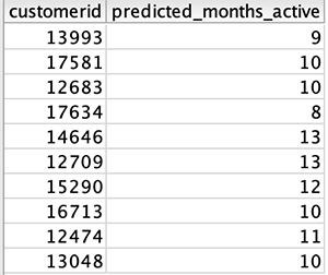
Now let’s run a query to see which customers qualify for our customer loyalty program by being active for at least 7 months:

select 
  customerid,  
  predict_customer_activity(customerid, country, stockcode, description, invoicedate, sales_amt) as predicted_months_active
  from ecommerce_sales_prediction
 where predicted_months_active >=7
 group by 1,2
 limit 10;

The following table shows our output.

Redshift ML now supports Prediction Probabilities for classification models. For classification problem in machine learning, for a given record, each label can be associated with a probability that indicates how likely this record really belongs to the label. With option to have probabilities along with the label, customers could use the classification results when confidence based on chosen label is higher than a certain threshold value returned by the model.

Prediction probabilities are calculated by default for classification models and an additional function is created while creating model without impacting performance of the ML model.

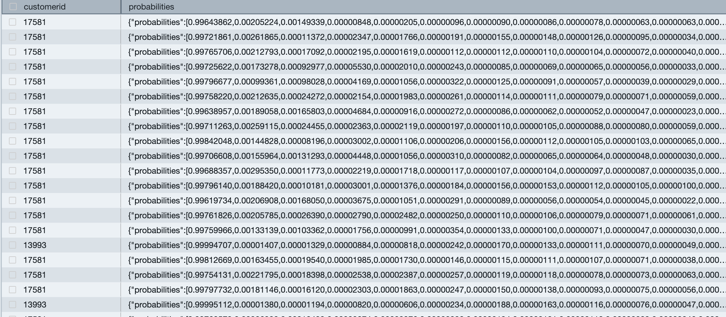
Now let’s run the query to use the prediction probabilities function by using the new function – predict_customer_activity_prod. Prediction probabilities provides label prediction based on the value which helps understand probability of the prediction.

Run the following query for one customer to see the probability output:

select 
customerid,
predict_customer_activity_prob(customerid, country, stockcode, description, invoicedate, sales_amt) as probabilities
 from ecommerce_sales_prediction
where customerid in (13993, 17581)
group by 1,2;

This query results shows prediction probabilities for all 13 labels (or classes) for these two accounts in the multi-classification model. We have multiple rows since a given customer may have multiple purchases.

Let’s run below query to get label and prediction probabilities values of the first label for these two customers. As you can see label denotes nbr_of_months and probabilities column values show confidence of label value.

Select t1.customerid, prediction.labels[0], prediction.probabilities[0]
from (select
customerid,
predict_customer_activity_prob(customerid, country, stockcode, description, invoicedate, sales_amt) as prediction
from ecommerce_sales_prediction
where customerid in(13993, 17581)
)t1
group by 1,2,3
order by 1;

Now you can run a query to get prediction probability to two decimal places which could be useful when using this value for setting the threshold and using it to decide if label should be used.

Select t1.customerid, prediction.labels[0] as labels, cast(prediction.probabilities[0] as decimal(4,2)) as probabilities
from (select
customerid,
predict_customer_activity_prob(customerid, country, stockcode, description, invoicedate, sales_amt) as prediction
from ecommerce_sales_prediction
where customerid in(13993, 17581)
)t1
group by 1,2,3
order by 1;

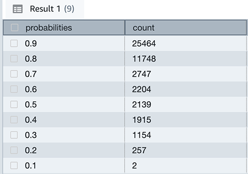
It is important to validate the model using prediction probabilities by running on whole inference data set and see the percentile. This helps in determining thresholds when to use predicted label with higher degree of confidence. You can run below query to calculate probabilities with total counts on whole inference data set to understand how many customers the active months label lies in probabilities percentile.

Select cast(prediction.probabilities[0] as decimal(4,1)) as probabilities, count(*) 
from (select 
  customerid,
  predict_customer_activity_prob(customerid, country, stockcode, description, invoicedate, sales_amt) as prediction
  from ecommerce_sales_prediction
)t1
group by 1
order by 1 desc;

Redshift ML is able to identify the right combination of features to come up with a usable prediction model with Model Explainability. It helps explain how these models make predictions using a feature attribution approach which in turn helps improve your ML models. We can check impact of each attribute and its contribution and weightage in the model selection using the following command:

select json_table.report.explanations.kernel_shap.label0.global_shap_values
from (select explain_model('ecommerce_customer_activity') as report) as json_table;

The following output is from the above command, where each attribute weightage is representative of its role in the model decision-making.

{"country":0.7581221856672759,"customerid":5.145962460036875,"description":0.14511538769719449,"invoicedate":1.8507790560421705,"sales_amt":0.9581555063586144,"stockcode":0.14785739737248208}	

Troubleshooting

Although the Create Model statement in Amazon Redshift automatically takes care of initiating the SageMaker Autopilot process to build, train, and tune the best ML model and deploy that model in Amazon Redshift, you can view the intermediate steps performed in this process, which may also help you with troubleshooting if something goes wrong. You can also retrieve the AutoML Job Name from the output of the show model command.

While creating the model, you need to mention an Amazon Simple Storage Service (Amazon S3) bucket name as the value for parameter, s3_bucket. You use this bucket to share training data and artifacts between Amazon Redshift and SageMaker. Amazon Redshift creates a subfolder in this bucket prior to unload of the training data. When training is complete, it deletes the subfolder and its contents unless you set the parameter s3_garbage_collect to off, which you can use for troubleshooting purposes. For more information, see CREATE MODEL.

For information about using the SageMaker console and Amazon SageMaker Studio, see Build regression models with Amazon Redshift ML.

Conclusion

Amazon Redshift ML provides the right platform for database users to create, train, and tune models using a SQL interface. In this post, we walked you through how to create a multi-class classification model. We hope you can take advantage of Amazon Redshift ML to help gain valuable insights.

For more information about building different models with Amazon Redshift ML, see Build regression models with Amazon Redshift ML  and read the Amazon Redshift ML documentation.

Acknowledgments

Per the UCI Machine Learning Repository, this data was made available by Dr Daqing Chen, Director: Public Analytics group. chend ‘@’ lsbu.ac.uk, School of Engineering, London South Bank University, London SE1 0AA, UK.

Dua, D. and Graff, C. (2019). UCI Machine Learning Repository [http://archive.ics.uci.edu/ml]. Irvine, CA: University of California, School of Information and Computer Science.

About the Authors

Phil Bates is a Senior Analytics Specialist Solutions Architect at AWS with over 25 years of data warehouse experience.

Debu Panda, a principal product manager at AWS, is an industry leader in analytics, application platform, and database technologies and has more than 25 years of experience in the IT world.

Nikos Koulouris is a Software Development Engineer at AWS. He received his PhD from University of California, San Diego and he has been working in the areas of databases and analytics.

Enrico Sartorello is a Sr. Software Development Engineer at Amazon Web Services. He helps customers adopt machine learning solutions that fit their needs by developing new functionalities for Amazon SageMaker. In his spare time, he passionately follows his soccer team and likes to improve his cooking skills.

Rohit Bansal is an Analytics Specialist Solutions Architect at AWS. He specializes in Amazon Redshift and works with customers to build next-generation analytics solutions using other AWS Analytics services.