AWS Machine Learning Blog

Automatically detect sports highlights in video with Amazon SageMaker

July 2023: Please refer to the Media Replay Engine (MRE) solution presented in this Github repo instead, for the latest and more efficient solution for this use case. MRE is a framework for building automated video clipping and replay (highlight) generation pipelines using AWS services for live and video-on-demand (VOD) content.

Extracting highlights from a video is a time-consuming and complex process. In this post, we provide a new take on instant replay for sporting events using a machine learning (ML) solution for automatically creating video highlights from original video content. Video highlights are then available for download so that users can continue to view them via a web app.

We use Amazon SageMaker to analyze a full-length sports video (in our case, a soccer match) and tag segments of the original video that are highlights (penalty kicks). We also show how to apply our end-to-end architecture to not only other sports, but other types of videos, given the availability of appropriate training data.

Architecture overview

The following diagram depicts our solution architecture.

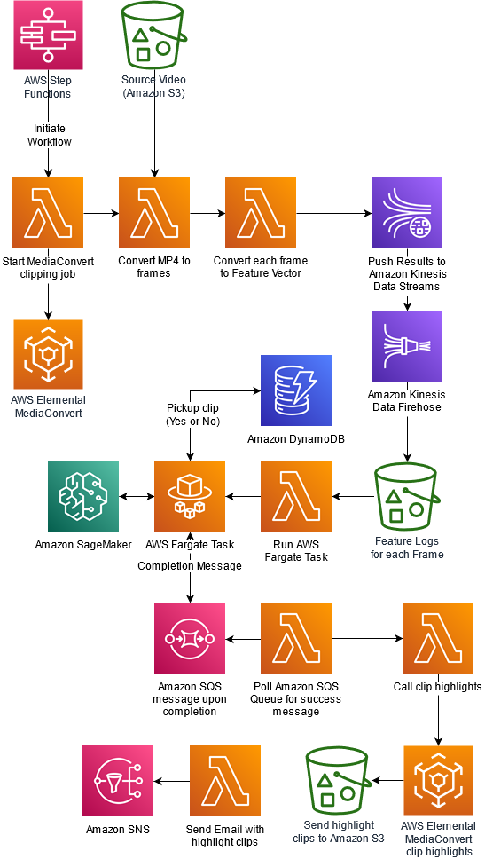
Orchestration overview

We use AWS Lambda functions as part of the following AWS Step Functions workflow to orchestrate a series of AWS Lambda functions for each step of the process.

The first step of the workflow is to start a MediaConvert job that breaks down the video into individual frames. Once the MediaConvert job completes, a Lambda Function converts each frame to a feature vector. The Lambda function generates feature vectors by passing individual images through a pretrained model (Inception V3). These feature vectors are then sent as topics via Amazon Kinesis Data Streams and Amazon Kinesis Data Firehose, and are finally stored in Amazon S3. Next step of the workflow is to invoke a machine learning model to infer if a video segment is interesting enough to pick up based on the sequence of feature vectors. The model determines what actions defined in the UCF101 labels are seen in the video. Here, AWS Fargate acts as a driver that loops through all sequences of feature vectors, prepares them for inference, performs inference using a SageMaker endpoint, and then collates results in an Amazon DynamoDB table. After the Fargate task completes, a message is placed in an Amazon SQS queue. A Lambda function periodically polls this Amazon SQS queue. When a completion message is detected, the Lambda function triggers a MediaConvert job to prepare highlight segments based on the results of machine learning inference. Finally, an email containing links to highlight clips is sent to the email address specified by the user.

Methodology

We use deep learning techniques to identify an activity in a given video. We use a deep Convolutional Neural Network (CNN) based on a pretrained Inception V3 model—to generate features from images extracted from video, and use a LSTM (Long Short-Term memory) network for predicting actions from sequences of features. Both CNN and LSTM are types of neural networks used in ML-based computer vision solutions. Let’s briefly discuss neural networks and related terms before we jump into 2D-CNN and LSTM.

Neural networks

Neural networks are computer systems vaguely inspired by biological neural networks that constitute animal brains. Just like how the basic unit of the brain is the neuron, the building block of an artificial neural network is a perceptron. Perceptrons do very simple processing. Perceptrons are connected to a large meshed network, which forms a neural network. The neural networks are organized into layers and connections between them are weighted. A neural network isn’t an algorithm, it’s a framework that multiple different ML algorithms can use. We describe different layers in a CNN later in this post when we build a model for extracting features from images extracted from videos.

A neural network is a supervised learning technique in ML. This means that model get better and better as it sees more similar objects, so more training samples results in a better accuracy.

Let’s break down the terms in deep CNNs and understand why this technique is effective in an image recognition. Together with LSTM, we use this technique later for activity identification in a given video.

Deep Convolutional Neural Networks

Deep Convolutional Neural Networks such as Inception V3 and YOLOV5 have proven to be a very effective technique for image recognition and other downstream fine-tuning tasks. More recent vision-transformer based models are also currently being used for state-of-the-art image classification, object detection and segmentation masks. Image recognition has many applications. Something that started as a technique to improve the accuracy of human written digits has evolved to solve more complex problems such as identifying and labeling specific objects and backgrounds in an image.

Although deep CNNs have made the problem of image classification and identification simple and improved the accuracy of results significantly, the implementation of an end-to-end solution from scratch is not a simple task. We recommend using services such as Amazon Rekognition, which provides a state-of-the-art API-based solution for image classification and image recognition solutions. If a custom model is required for solving computer vision problem for either image or video, SageMaker provides a framework for training and inference. SageMaker provides support for multiple ML frameworks using BYOC (bring your own container). We use BYOC in SageMaker for Keras to develop a model for activity recognition and deploy the model for inference.

The convolution technique makes the output of neural networks more robust and accurate because instead of processing every image as a single tile of pixels, it breaks an image into multiple tiles using a sliding window of fixed size. Each tile activates the next layer separately, and all tiles of an image are aggregated in successive layers to generate an output. For example, this allows the digit 8 in the left corner of an image to be identified as the same digit 8 in the right corner of an image. This is a called translation invariance.

LSTM

LSTM networks are types of Recurrent Neural Networks (RNNs), which contain special cells or neurons that allow information to persist due the existence of loops or special memory units. LSTMs in particular are useful in learning tasks involving time sequences of data (like our use case of video classification, which is a time sequence of static frames), especially when there is a need to remember information for long periods of time.

Challenges with video processing

It’s important to keep in mind that videos are like a flip book. The static image on each page when flipped generates the perception of motion. The faster you flip, the better the quality of motion perception you get.

Images are stored as a stream of pixels in a 2D spatial arrangement. This is how a computer program reads images. As an extension of images, videos have an extra dimension of time. Videos are a time series of static images. This makes videos a 3D spatial and temporal arrangement of pixels.

The extra dimension requires more compute and memory to develop an ML model. A lot of preprocessing is required before we can feed video input into CNNs and LSTM.

Apart from increased complexity in preprocessing and processing, there is also the lack of open datasets available for research on video data.

In this post, we use samples provided in the UCF101 dataset for building a model and deploying an endpoint for inference.

Reading a video and extracting frames

Assume that the video source that we’re analyzing in order to extract highlights is in Amazon Simple Storage Service (Amazon S3). We use AWS Elemental MediaConvert to split the video into individual frames, and this MediaConvert job is triggered from the following Lambda function:

1.	import json  
2.	import boto3  
3.	  
4.	s3_location = 's3://<ARTIFACT-BUCKET>/BYUfootballmatch.mp4'  
5.	  
6.	  
7.	def lambda_handler(event, context):  
8.	    with open('mediaconvert.json') as f:  
9.	        data = json.load(f)  
10.	      
11.	    client = boto3.client('mediaconvert')  
12.	    endpoint = client.describe_endpoints()['Endpoints'][0]['Url']  
13.	      
14.	    myclient = boto3.client('mediaconvert', endpoint_url=endpoint)  
15.	  
16.	    
17.	  
18.	    data['Settings']['Inputs'][0]['FileInput'] = s3_location  
19.	      
20.	    response = myclient.create_job(  
21.	    Queue=data['Queue'],  
22.	    Role=data['Role'],  
23.	    Settings=data['Settings'])  
24.	      

Line 22 uses the AWS SDK for Python (Boto3) to initiate the MediaConvert client using the following JSON template. You can specify codec settings, width, height, and other parameters specific to your video format.

1.	{  
2.	  "Queue": "arn:aws:mediaconvert:<REGION>:<AWS ACCOUNT NUMBER>:queues/Default",  
3.	  "UserMetadata": {},  
4.	  "Role": "arn:aws:iam::<AWS ACCOUNT ID>:role/MediaConvertRole",  
5.	  "Settings": {  
6.	    "OutputGroups": [  
7.	      {  
8.	        "CustomName": "MP4",  
9.	        "Name": "File Group",  
10.	        "Outputs": [  
11.	          {  
12.	            "ContainerSettings": {  
13.	              "Container": "MP4",  
14.	              "Mp4Settings": {  
15.	                "CslgAtom": "INCLUDE",  
16.	                "FreeSpaceBox": "EXCLUDE",  
17.	                "MoovPlacement": "PROGRESSIVE_DOWNLOAD"  
18.	              }  
19.	            },  
20.	            "VideoDescription": {  
21.	              "Width": 1280,  
22.	              "ScalingBehavior": "DEFAULT",  
23.	              "Height": 720,  
24.	              "TimecodeInsertion": "DISABLED",  
25.	              "AntiAlias": "ENABLED",  
26.	              "Sharpness": 50,  
27.	              "CodecSettings": {  
28.	                "Codec": "H_264",  
29.	                "H264Settings": {  
30.	                  "InterlaceMode": "PROGRESSIVE",  
31.	                  "NumberReferenceFrames": 3,  
32.	                  "Syntax": "DEFAULT",  
33.	                  "Softness": 0,  
34.	                  "GopClosedCadence": 1,  
35.	                  "GopSize": 90,  
36.	                  "Slices": 1,  
37.	                  "GopBReference": "DISABLED",  
38.	                  "SlowPal": "DISABLED",  
39.	                  "SpatialAdaptiveQuantization": "ENABLED",  
40.	                  "TemporalAdaptiveQuantization": "ENABLED",  
41.	                  "FlickerAdaptiveQuantization": "DISABLED",  
42.	                  "EntropyEncoding": "CABAC",  
43.	                  "Bitrate": 3000000,  
44.	                  "FramerateControl": "INITIALIZE_FROM_SOURCE",  
45.	                  "RateControlMode": "CBR",  
46.	                  "CodecProfile": "MAIN",  
47.	                  "Telecine": "NONE",  
48.	                  "MinIInterval": 0,  
49.	                  "AdaptiveQuantization": "HIGH",  
50.	                  "CodecLevel": "AUTO",  
51.	                  "FieldEncoding": "PAFF",  
52.	                  "SceneChangeDetect": "ENABLED",  
53.	                  "QualityTuningLevel": "SINGLE_PASS",  
54.	                  "FramerateConversionAlgorithm": "DUPLICATE_DROP",  
55.	                  "UnregisteredSeiTimecode": "DISABLED",  
56.	                  "GopSizeUnits": "FRAMES",  
57.	                  "ParControl": "INITIALIZE_FROM_SOURCE",  
58.	                  "NumberBFramesBetweenReferenceFrames": 2,  
59.	                  "RepeatPps": "DISABLED"  
60.	                }  
61.	              },  
62.	              "AfdSignaling": "NONE",  
63.	              "DropFrameTimecode": "ENABLED",  
64.	              "RespondToAfd": "NONE",  
65.	              "ColorMetadata": "INSERT"  
66.	            },  
67.	            "AudioDescriptions": [  
68.	              {  
69.	                "AudioTypeControl": "FOLLOW_INPUT",  
70.	                "CodecSettings": {  
71.	                  "Codec": "AAC",  
72.	                  "AacSettings": {  
73.	                    "AudioDescriptionBroadcasterMix": "NORMAL",  
74.	                    "Bitrate": 96000,  
75.	                    "RateControlMode": "CBR",  
76.	                    "CodecProfile": "LC",  
77.	                    "CodingMode": "CODING_MODE_2_0",  
78.	                    "RawFormat": "NONE",  
79.	                    "SampleRate": 48000,  
80.	                    "Specification": "MPEG4"  
81.	                  }  
82.	                },  
83.	                "LanguageCodeControl": "FOLLOW_INPUT"  
84.	              }  
85.	            ]  
86.	          }  
87.	        ],  
88.	        "OutputGroupSettings": {  
89.	          "Type": "FILE_GROUP_SETTINGS",  
90.	          "FileGroupSettings": {  
91.	            "Destination": "s3://<ARTIFACT-BUCKET>/MP4/"  
92.	          }  
93.	        }  
94.	      },  
95.	      {  
96.	        "CustomName": "Thumbnails",  
97.	        "Name": "File Group",  
98.	        "Outputs": [  
99.	          {  
100.	            "ContainerSettings": {  
101.	              "Container": "RAW"  
102.	            },  
103.	            "VideoDescription": {  
104.	              "Width": 768,  
105.	              "ScalingBehavior": "DEFAULT",  
106.	              "Height": 576,  
107.	              "TimecodeInsertion": "DISABLED",  
108.	              "AntiAlias": "ENABLED",  
109.	              "Sharpness": 50,  
110.	              "CodecSettings": {  
111.	                "Codec": "FRAME_CAPTURE",  
112.	                "FrameCaptureSettings": {  
113.	                  "FramerateNumerator": 20,  
114.	                  "FramerateDenominator": 1,  
115.	                  "MaxCaptures": 10000000,  
116.	                  "Quality": 100  
117.	                }  
118.	              },  
119.	              "AfdSignaling": "NONE",  
120.	              "DropFrameTimecode": "ENABLED",  
121.	              "RespondToAfd": "NONE",  
122.	              "ColorMetadata": "INSERT"  
123.	            }  
124.	          }  
125.	        ],  
126.	        "OutputGroupSettings": {  
127.	          "Type": "FILE_GROUP_SETTINGS",  
128.	          "FileGroupSettings": {  
129.	            "Destination": "s3://<ARTIFACT-BUCKET>/Thumbnails/"  
130.	          }  
131.	        }  
132.	      }  
133.	    ],  
134.	    "AdAvailOffset": 0,  
135.	    "Inputs": [  
136.	      {  
137.	        "AudioSelectors": {  
138.	          "Audio Selector 1": {  
139.	            "Offset": 0,  
140.	            "DefaultSelection": "DEFAULT",  
141.	            "ProgramSelection": 1  
142.	          }  
143.	        },  
144.	        "VideoSelector": {  
145.	          "ColorSpace": "FOLLOW"  
146.	        },  
147.	        "FilterEnable": "AUTO",  
148.	        "PsiControl": "USE_PSI",  
149.	        "FilterStrength": 0,  
150.	        "DeblockFilter": "DISABLED",  
151.	        "DenoiseFilter": "DISABLED",  
152.	        "TimecodeSource": "EMBEDDED",  
153.	        "FileInput": "s3:// <ARTIFACT-BUCKET>/BYUfootballmatch.mp4"  
154.	      }  
155.	    ]  
156.	  }  
157.	}  

While the MediaConvert job is running, another Lambda function checks for job completion. This function is written as follows:

1.	import json  
2.	import boto3  
3.	import pprint   
4.	def lambda_handler(event, context):  
5.	      
6.	    client = boto3.client('mediaconvert')  
7.	    endpoint = client.describe_endpoints()['Endpoints'][0]['Url']  
8.	      
9.	    myclient = boto3.client('mediaconvert', endpoint_url=endpoint)  
10.	      
11.	    response = myclient.list_jobs(  
12.	    MaxResults=1,  
13.	    Order='DESCENDING')  
14.	      
15.	    #Status='SUBMITTED'|'PROGRESSING'|'COMPLETE'|'CANCELED'|'ERROR')  
16.	    print(len(response['Jobs']))  
17.	    Status = response['Jobs'][0]['Status']  
18.	    Id = response['Jobs'][0]['Id']  
19.	    print(Id, Status)  
20.	    

Collect feature vectors for training

Each frame is passed through a pre-trained InceptionV3 model to extract features. The model is small enough to be packaged within the Lambda function along with an ML framework that was used to train the model (MXNet). We don’t describe the image classification model training here, but the overall procedure to do this is as follows:

  1. Train the InceptionV3 network on MXNet using ILSVRC 2012 data. For details about the network architecture and the dataset, see Rethinking the Inception Architecture for Computer Vision.
  2. Load the trained model into a Lambda function (model.json and model.params files) and pop the final layer. We’re left with an output layer that doesn’t perform classification, but provides us with a feature vector of size 1024×1.
  3. Each time a frame is passed through the Lambda function, it outputs this feature vector into a data stream, via Amazon Kinesis Data Streams.
  4. Topics from this stream are collected using Amazon Kinesis Data Firehose and output into another S3 bucket.
  5. An AWS Fargate job orders the files based on the original order in which the frames appear. Because we trigger 1,000 instances of this Lambda function in parallel with one frame per function, the outputs can be slightly out of order. You can also use SageMaker processing instead of Fargate. This gives us our final training data, which we can use in our SageMaker custom video classification model that can identify groups of frames as highlights. In our example, the highlights in our soccer video are penalty kicks.

The code for this Lambda function is as follows:

1.	import logging  
2.	import boto3  
3.	import json  
4.	import numpy as np  
5.	import tempfile  
6.	  
7.	logger = logging.getLogger()  
8.	logger.setLevel(logging.INFO)  
9.	region =   
10.	relevant_timestamps = []  
11.	  
12.	import mxnet as mx  
13.	  
14.	  
15.	def load_model(s_fname, p_fname):  
16.	    """ 
17.	    Load model checkpoint from file. 
18.	    :return: (arg_params, aux_params) 
19.	    arg_params : dict of str to NDArray 
20.	        Model parameter, dict of name to NDArray of net's weights. 
21.	    aux_params : dict of str to NDArray 
22.	        Model parameter, dict of name to NDArray of net's auxiliary states. 
23.	    """  
24.	    symbol = mx.symbol.load(s_fname)  
25.	    save_dict = mx.nd.load(p_fname)  
26.	    arg_params = {}  
27.	    aux_params = {}  
28.	    for k, v in save_dict.items():  
29.	        tp, name = k.split(':', 1)  
30.	        if tp == 'arg':  
31.	            arg_params[name] = v  
32.	        if tp == 'aux':  
33.	            aux_params[name] = v  
34.	    return symbol, arg_params, aux_params  
35.	  
36.	sym, arg_params, aux_params = load_model('model2.json', 'model2.params')  
37.	  
38.	#load json and params into model  
39.	#mod = None  
40.	  
41.	# We bind the module with the input shape and specify that it is only for predicting. The number 1 added before the image shape (3x224x224) means that we will only predict one image at a tim  
42.	  
43.	# FULL MODEL  
44.	#mod = mx.mod.Module(symbol=sym, label_names=None)  
45.	#mod.bind(for_training=False, data_shapes=[('data', (1,3,224,224))], label_shapes=mod._label_shapes)  
46.	#mod.set_params(arg_params, aux_params, allow_missing=True)  
47.	  
48.	  
49.	from collections import namedtuple  
50.	Batch = namedtuple('Batch', ['data'])  
51.	  
52.	def lambda_handler(event, context):  
53.	    # PARTIAL MODEL  
54.	    mod2 = None  
55.	    all_layers = sym.get_internals()  
56.	    print(all_layers.list_outputs()[-10:])  
57.	    sym2 = all_layers['global_pool_output']  
58.	    mod2 = mx.mod.Module(symbol=sym2,label_names=None)  
59.	    #mod2.bind(for_training=False, data_shapes = [('data', (1,3,224,224))], label_shapes = mod2._label_shapes)  
60.	    mod2.bind(for_training=False, data_shapes=[('data', (1,3,299,299))])  
61.	    mod2.set_params(arg_params, aux_params)  
62.	      
63.	    #Get image(s) from s3  
64.	    s3 = boto3.resource('s3')  
65.	    bucket = s3.Bucket(event['bucketname'])  
66.	    object = bucket.Object(event['filename'])  
67.	  
68.	    #img = mx.image.imread('image.jpg')  
69.	      
70.	    tmp = tempfile.NamedTemporaryFile()  
71.	    with open(tmp.name, 'wb') as f:  
72.	        object.download_fileobj(f)  
73.	        img=mx.image.imread(tmp.name)  
74.	        # convert into format (batch, RGB, width, height)   
75.	        img = mx.image.imresize(img, 299, 299) # resize  
76.	        img = img.transpose((2, 0, 1)) # Channel first  
77.	        img = img.expand_dims(axis=0) # batchify  
78.	      
79.	        mod2.forward(Batch([img]))  
80.	    out = np.squeeze(mod2.get_outputs()[0].asnumpy())  
81.	      
82.	    kinesis_client = boto3.client('kinesis')  
83.	    put_response = kinesis_client.put_record(StreamName = 'bottleneck_stream',Data = json.dumps({'filename':event['filename'],'features':out.tolist()}), PartitionKey = "partitionkey")  
84.	    return 'Wrote features to kinesis stream'  

Label the images for training the model

As mentioned earlier, we use the UCF101 action recognition dataset, which you can obtain from within a Jupyter notebook instance using the following command:

!wget http://crcv.ucf.edu/data/UCF101/UCF101.rar

We extract the same feature vectors from InceptionV3 for all action recognition datasets contained within the .rar file downloaded (it contains several examples of 101 different actions, including ones relevant for our soccer example, such as the soccer penalty and soccer juggling labels.

We construct a custom LSTM model in TensorFlow and use features extracted in the previous step to train the model. The LSTM model is structured as follows:

  • Layer 1 – 2048 LSTM cells
  • Layer 2 – 512 Dense cells
  • Layer 3 – Drop out layer (p=0.5)
  • Layer 4 – Softmax layer for 101 classes

Model.summary() provides the following summary:

Layer (type)                 Output Shape              Param #   
=================================================================
lstm_1 (LSTM)                (None, 2048)              33562624  
_________________________________________________________________
dense_1 (Dense)              (None, 512)               1049088   
_________________________________________________________________
dropout_1 (Dropout)          (None, 512)               0         
_________________________________________________________________
dense_2 (Dense)              (None, 101)               51813     
=================================================================
Total params: 34,663,525
Trainable params: 34,663,525
Non-trainable params: 0
___________________________

With a more relevant dataset, you should only include the classes you require in the classification task. Due to the nature of the problem selected, we only had access to this open dataset. However, for extracting highlights from custom videos, you can use your own labeled video datasets.

We save the model using the following code in the notebook:

trainedmodel.save('lstm_model.h5')

We create a container containing the following code and Dockerfile, to host the model using SageMaker. The following is the Python entry point code for inference:

1.	#!/usr/bin/env python  
2.	from __future__ import print_function import os import sys import traceback import numpy as np import pandas as pd   
3.	import tensorflow as tf from keras.layers import Dropout, Dense from keras.wrappers.scikit_learn import   
4.	KerasClassifier from keras.models import Sequential from keras.models import load_model def train():  
5.	    print('Starting the training.')  
6.	    try:  
7.	        model = load_model('lstm_model.h5')  
8.	        print('Model is loaded ... Training is complete.')  
9.	    except Exception as e:  
10.	        # Write out an error file. This will be returned as the failure Reason in the DescribeTrainingJob result.  
11.	        trc = traceback.format_exc()  
12.	        with open(os.path.join(output_path, 'failure'), 'w') as s:  
13.	            s.write('Exception during training: ' + str(e) + '\n' + trc)  
14.	        # Printing this causes the exception to be in the training job logs  
15.	        print(  
16.	            'Exception during training: ' + str(e) + '\n' + trc,  
17.	            file=sys.stderr)  
18.	        # A non-zero exit code causes the training job to be marked as Failed.  
19.	        sys.exit(255) if __name__ == '__main__':  
20.	    train()  
21.	    # A zero exit code causes the job to be marked a Succeeded.  
22.	    sys.exit(0)  

We containerize and push the Docker image to Amazon Elastic Container Registry (Amazon ECR):

1.	%%sh  
2.	  
3.	# The name of our algorithm  
4.	algorithm_name=kerassample14  
5.	  
6.	cd container  
7.	  
8.	chmod +x keras-model/train  
9.	chmod +x keras-model/serve  
10.	  
11.	account=$(aws sts get-caller-identity --query Account --output text)  
12.	  
13.	# Get the region defined in the current configuration (default to us-west-2 if none defined)  
14.	region=$(aws configure get region)  
15.	region=${region:-us-west-2}  
16.	  
17.	fullname="${account}.dkr.ecr.${region}.amazonaws.com/${algorithm_name}:latest"  
18.	echo $fullname  
19.	# If the repository doesn't exist in ECR, create it.  
20.	  
21.	aws ecr describe-repositories --repository-names "${algorithm_name}" > /dev/null 2>&1  
22.	  
23.	if [ $? -ne 0 ]  
24.	then  
25.	    aws ecr create-repository --repository-name "${algorithm_name}" > /dev/null  
26.	fi  
27.	  
28.	# Get the login command from ECR and execute it directly  
29.	$(aws ecr get-login --region ${region} --no-include-email)  
30.	  
31.	# Build the docker image locally with the image name and then push it to ECR  
32.	# with the full name.  
33.	  
34.	docker build  -t ${algorithm_name} .  
35.	docker tag ${algorithm_name} ${fullname}  
36.	  
37.	docker push ${fullname} 

Lastly, we host the model on SageMaker:

1.	account = sess.boto_session.client('sts').get_caller_identity()['Account']  
2.	region = sess.boto_session.region_name  
3.	image = f'<account number>.dkr.<region>.amazonaws.com/<containername>:latest'  
4.	  
5.	classifier = sage.estimator.Estimator(  
6.	    image,   
7.	    role,   
8.	    1,   
9.	    'ml.c5.2xlarge',   
10.	    output_path="s3://{}/output".format(sess.default_bucket()),  
11.	    sagemaker_session=sess) 
12.	
13.	
14.	from sagemaker.predictor import csv_serializer
15.	predictor = classifier.deploy(1, 'ml.m5.xlarge', serializer=csv_serializer)

SageMaker provides us with an endpoint to call for predictions where the input is a set of feature vectors (example, 10 frames or images corresponds to a 10×1024 feature matrix), and the output is a probability distribution across the 101 UCF101 classes. We’re only interested in the soccer penalty class. For the purposes of this blog, we use the UCF101 dataset but for your own use cases, do take the time to research relevant action recognition datasets or pretrained models.

Extract highlights

In our architecture, the Fargate job calls the SageMaker estimator sequentially with a set of feature vectors and stores the decision to pick up a set of frames or not in an Amazon DynamoDB table. When the Fargate job is complete, another Lambda function (see the following code) uses the DynamoDB table to edit a clipping job definition and submit the same to a MediaConvert job. This MediaConvert job splits the original video into smaller sections where the desired class of action was identified. In our case, this was the soccer penalty kicks. These extracted videos are then made public for access from outside the account using a Boto3 command from within the same Lambda function.

1.	import json  
2.	import boto3  
3.	import time  
4.	from boto3.dynamodb.conditions import Key, Attr  
5.	import math   
6.	  
7.	s3_location = 's3://<ARTIFACT-BUCKET>/BYUfootballmatch.mp4'  
8.	  
9.	def start_mediaconvert_job(data, sec_in, sec_out):  
10.	    
11.	      
12.	    client = boto3.client('mediaconvert')  
13.	    endpoint = client.describe_endpoints()['Endpoints'][0]['Url']  
14.	      
15.	    myclient = boto3.client('mediaconvert', endpoint_url=endpoint)  
16.	  
17.	    data['Settings']['Inputs'][0]['FileInput'] = s3_location  
18.	      
19.	    starttime = time.strftime('%H:%M:%S:00', time.gmtime(sec_in))  
20.	    endtime = time.strftime('%H:%M:%S:00', time.gmtime(sec_out))  
21.	      
22.	    data['Settings']['Inputs'][0]['InputClippings'][0] = {'EndTimecode': endtime, 'StartTimecode': starttime}  
23.	      
24.	    data['Settings']['OutputGroups'][0]['Outputs'][0]['NameModifier'] = '-from-'+str(sec_in)+'-to-'+str(sec_out)  
25.	      
26.	    response = myclient.create_job(  
27.	    Queue=data['Queue'],  
28.	    Role=data['Role'],  
29.	    Settings=data['Settings'])  
30.	  
31.	def lambda_handler(event, context):  
32.	      
33.	    
34.	    dynamodb = boto3.resource('dynamodb')  
35.	    table = dynamodb.Table('sports-lstm-final-output')        
36.	    response = table.scan()             
37.	    timeins = []  
38.	    timeouts=[]        
39.	    for i in response['Items']:  
40.	        if(i['pickup']=='yes'):              
41.	            timeins.append(i['timein'])  
42.	            timeouts.append(i['timeout'])  
43.	              
44.	    timeins = sorted([int(x) for x in timeins])  
45.	    timeouts =sorted([int(x) for x in timeouts])      
46.	    mintime =min(timeins)  
47.	    maxtime =max(timeouts)  
48.	      
49.	    print('mintime='+str(mintime))  
50.	    print('maxtime='+str(maxtime))  
51.	      
52.	    print(timeins)  
53.	    print(timeouts)  
54.	    mystarttime = mintime  
55.	   
56.	    #find continuous range  
57.	    ranges = {}  
58.	    maxisofar=0  
59.	    rangecount = 0  
60.	    lastnum = timeouts[0]  
61.	    for i in range(len(timeins)-1):  
62.	        c=0  
63.	        if(timeouts[i] >= lastnum):  
64.	            for j in range(i,len(timeouts)-1):  
65.	                if(timeins[j+1] - timeins[j] == 20 and timeouts[j] - timeins[i] == 40 + c*20 ):  
66.	                    c=c+1  
67.	                    continue  
68.	                if(timeins[i+1] - timeins[i] > 20 and timeouts[j] - timeins[i] == 40 ):  
69.	                    print('single frame',i,j)  
70.	                    ranges[rangecount] = {'start':timeins[i], 'end':timeouts[i], 'count':1}   
71.	                    rangecount=rangecount+1  
72.	                    lastnum = timeouts[i+1]  
73.	                    continue  
74.	                      

75.	            if(c>0):  
76.	                
77.	                ranges[rangecount] = {'start':timeins[i], 'end':timeouts[i+c], 'count':c}  
78.	                rangecount=rangecount+1  
79.	                lastnum = timeouts[i+c+1]  
80.	  
81.	    print(lastnum)  
82.	    if(lastnum == timeouts[-1]):  
83.	        # Last frame is a single frame  
84.	        ranges[rangecount] = {'start':timeins[-1], 'end':timeouts[-1], 'count':1}   
85.	          
86.	    print(ranges)  
87.	    #Find max continuous range  
88.	    maxc = 0  
89.	    maxi = 0  
90.	    for i in range(len(ranges)):  
91.	        if maxc < ranges[i]['count']:  
92.	            maxi = i  
93.	            maxc = ranges[i]['count']  
94.	    buffer = 1 #seconds  
95.	      
96.	   
97.	    with open('mediaconvert.json') as f:  
98.	        data = json.load(f)  
99.	      
100.	    # DO THIS for ALL RANGES  
101.	    for i in range(len(ranges)):  
102.	        if ranges[i]['count']:  
103.	            sec_in = math.floor(ranges[i]['start']/20.0) - buffer  
104.	            sec_out = math.ceil(ranges[i]['end']/20.0) + buffer #20:1 was the framer rate in original video  
105.	            sec_in = 0 if sec_in<0 else sec_in  
106.	            start_mediaconvert_job(data, sec_in, sec_out)  
107.	            time.sleep(1)  
108.	      
109.	    print(ranges)  
110.	    return json.dumps({'bucket':'elemental-media-input','prefix':'High','postfix':'mp4'}) 

Deployment Prerequisites

To deploy this solution, you will need to create an Amazon S3 bucket and designate it as an ARTIFACT-BUCKET. This bucket will be used for storing the video file as well as the model artifacts. You could run the follow AWS CLI command to create an Amazon S3 bucket:

aws s3api create-bucket   --bucket <ARTIFACT-BUCKET>

Next, un the following command to copy required artifacts to the artifact bucket.

aws s3 cp s3://aws-ml-blog/artifacts/sportshighlights/ \
s3://<ARTIFACT-BUCKET>  --recursive --copy-props none

Deploy the solution using AWS CloudFormation

We provide an AWS CloudFormation template for creating resources and setting up the workflow for this post. AWS CloudFormation enables you to model, provision, and manage AWS resources by treating infrastructure as code.

The CloudFormation template requires you to provide an email address that is used for sending links to highlight clips at the end of the workflow. The stack sets up the following resources:

Follow these steps to deploy this in your own account:

  1. Choose Launch Stack:

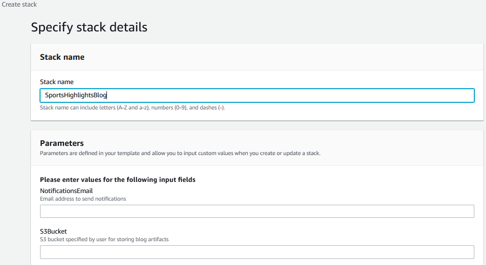
  1. Enter a name for the stack.
  2. Enter an email address where you choose to receive notifications from the Step Functions workflow.
  3. For S4Bucket, enter the name of the ARTIFACT-BUCKET that you created earlier.
  4. Choose Next.
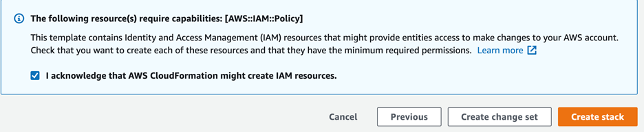
  5. On the Review page, select I acknowledge that AWS CloudFormation might create IAM resources.
  6. Choose Create stack.

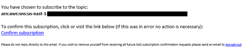
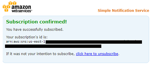
After the stack is successfully created, you will receive an email with a request to subscribe to the topic. Chose ‘Confirm subscription’.

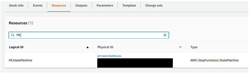
  1. From the AWS CloudFormation console, navigate to the resources tab for the stack you created. Click on the hyperlink (Physical ID) for the MLStateMachine resource.

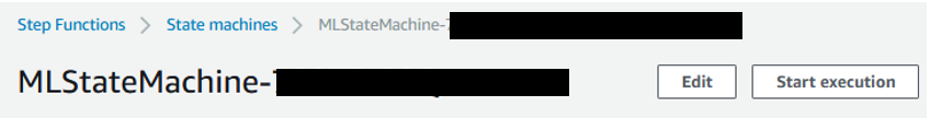
This should navigate you to the Step Functions console. Select ‘Start Execution’.

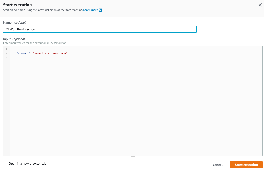
  1. Enter a name, select defaults for input and select ‘Start Execution’.

You can monitor progress of the Step Functions execution by navigating to the ‘Graph Inspector’.

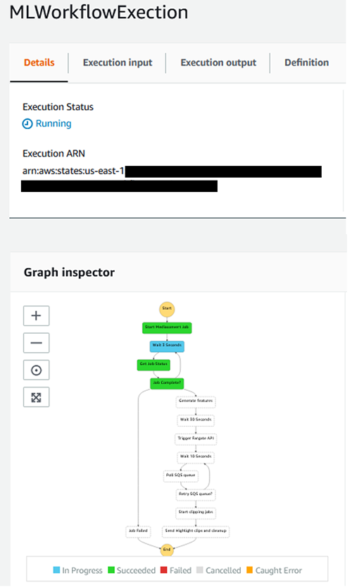
Wait for the Step Functions workflow to complete.

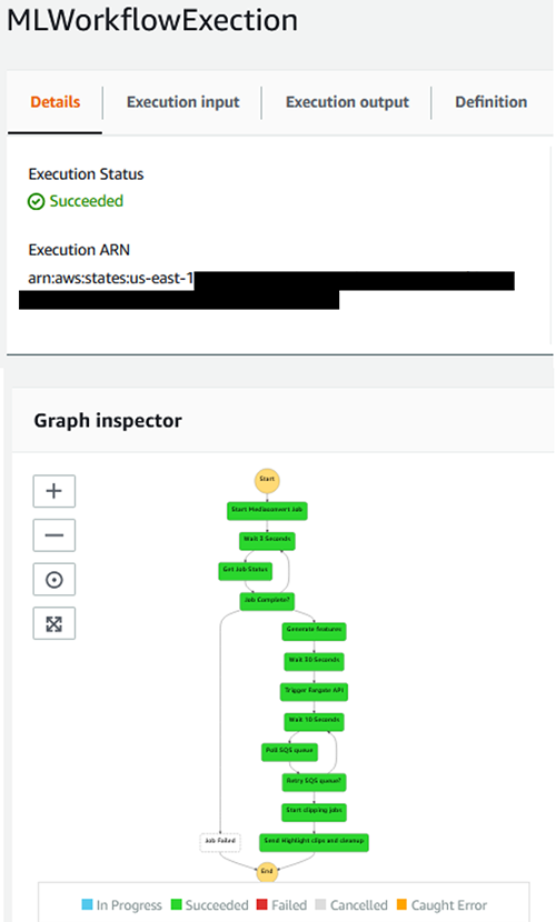
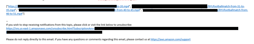
After the Step Functions execution completes, you should receive an email with Amazon S3 files representing the highlight clips from the original video. Following best practices, we do not expose these highlight clips publicly. You could navigate to the Amazon S3 bucket you created and will find the clips in a folder named HighLightclips.

At the end of the process, you should see that the following input video:

generates the following output highlight clip of a penalty kick:

Clean up

To avoid incurring ongoing charges, clean up your infrastructure by deleting the stack from the AWS CloudFormation console.

Empty the artifact bucket that you created for the blog. You could run the following AWS CLI command:

aws s3 rm s3://<ARTIFACT-BUCKET> --recursive 
aws s3api delete-bucket --bucket <ARTIFACT-BUCKET>

After this, navigate to AWS CloudFormation in AWS Management Console, select the stack you created and select ‘Delete’.

Conclusion

In this post, we showed you how to use a custom SageMaker model to generate sports highlights from full-length sports videos. You can extend this solution to generate highlights containing slam dunks, touch downs, home runs or sixers from your favorite sports videos, or from other shows, movies, meetings, and any other content in a video format – as long as you have a pretrained model, or you train a model specific to your use case.

For more information about how to make preprocessing easier, check out Amazon SageMaker Processing.

For more information about how to fine-tune state-of-the-art action recognition models like PAN Resnet 101, TSM, and R2+1D BERT, or host them on SageMaker as endpoints, see Deploy a Model in Amazon SageMaker.


About the Authors

Shreyas Subramanian is an AI/ML specialist Solutions Architect, and helps customers by using Machine Learning to solve their business challenges on the AWS Cloud.

Mohit Mehta is a leader in the AWS Professional Services Organization with expertise in AI/ML and Big Data technologies. Mohit holds a M.S in Computer Science, all 12 AWS certifications, MBA from College of William and Mary and GMP from Michigan Ross School of Business.

Vikrant Kahlir is Principal Architect in the Solutions Architecture team. He works with AWS strategic customers product and engineering teams to help them with technology solutions using AWS services for Managed Databases, AI/ML, HPC, Autonomous Computing, and IoT.