Category: Amazon Redshift
Amazon Redshift Spectrum – Exabyte-Scale In-Place Queries of S3 Data
Now that we can launch cloud-based compute and storage resources with a couple of clicks, the challenge is to use these resources to go from raw data to actionable results as quickly and efficiently as possible.
Amazon Redshift allows AWS customers to build petabyte-scale data warehouses that unify data from a variety of internal and external sources. Because Redshift is optimized for complex queries (often involving multiple joins) across large tables, it can handle large volumes of retail, inventory, and financial data without breaking a sweat. Once the data is loaded, our customers can make use of a plethora of enterprise reporting and business intelligence tools provided by the Redshift Partners.
One of the most challenging aspects of running a data warehouse involves loading data that is continuously changing and/or arriving at a rapid pace. In order to provide great query performance, loading data into a data warehouse includes compression, normalization, and optimization steps. While these steps can be automated and scaled, the loading process introduces overhead and complexity, and also gets in the way of those all-important actionable results.
Data formats present another interesting challenge. Some applications will process the data in its original form, outside of the data warehouse. Others will issue queries to the data warehouse. This model leads to storage inefficiencies because the data must be stored twice, and can also mean that results from one form of processing may not align with those from another due to delays introduced by the loading process.
Amazon Redshift Spectrum
In order to allow you to process your data as-is, where-is, while taking advantage of the power and flexibility of Amazon Redshift, we are launching Amazon Redshift Spectrum. You can use Spectrum to run complex queries on data stored in Amazon Simple Storage Service (S3), with no need for loading or other data prep.
You simply create a data source and issue your queries to your Redshift cluster as usual. Behind the scenes, Spectrum scales to thousands of instances on a per-query basis, ensuring that you get fast, consistent performance even as your data set grows up to an beyond an exabyte! Being able to query data stored in S3 means that you can scale your compute and your storage independently, with the full power of the Redshift query model and all of the reporting and business intelligence tools at your disposal. Your queries can reference any combination of data stored in Redshift tables and in S3.
When you issue a query, Redshift rips it apart and generates a query plan that minimizes the amount of S3 data that will be read, taking advantage of both column-oriented formats and data that is partitioned by date or another key. Then Redshift requests Spectrum workers from a large, shared pool and directs them to project, filter, and aggregate the S3 data. The final processing is performed within the Redshift cluster and the results are returned to you.
Because Spectrum operates on data that is stored in S3, you can process the data using other AWS services such as Amazon EMR and Amazon Athena. You can also implement hybrid models where frequently queried data is kept in Redshift local storage and the rest is S3, or where dimension tables are in Redshift along with the recent portions of the fact tables, with older data in S3. In order to drive even higher levels of concurrency, you can point multiple Redshift clusters at the same stored data.
Spectrum supports open, common data types including CSV/TSV, Parquet, SequenceFile, and RCFile. Files can be compressed using GZip or Snappy, with other data types and compression methods in the works.
Spectrum in Action
In order to get some first-hand experience with Spectrum I loaded up a sample data set and ran some queries!
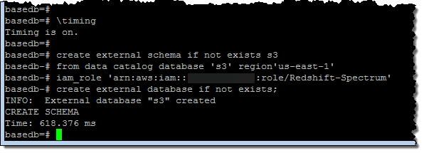
I started by creating an external schema and database:
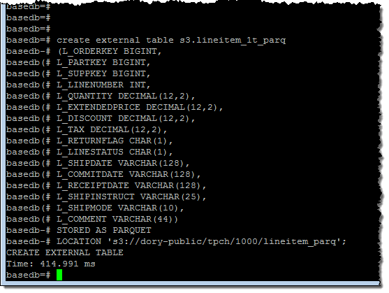
Then I created an external table within the database:
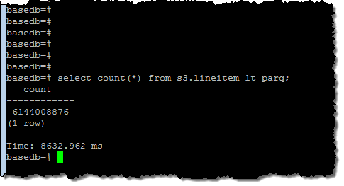
I ran a simple query to get a feel for the size of the data set (6.1 billion rows):
And then I ran a query that processed all of the rows:
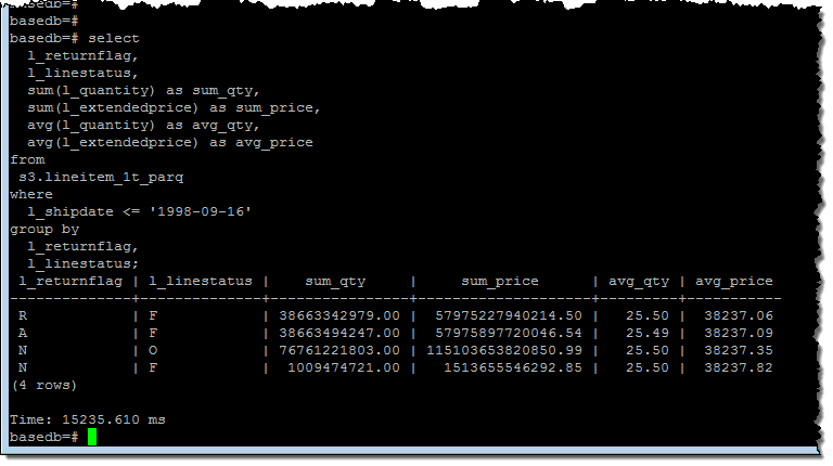
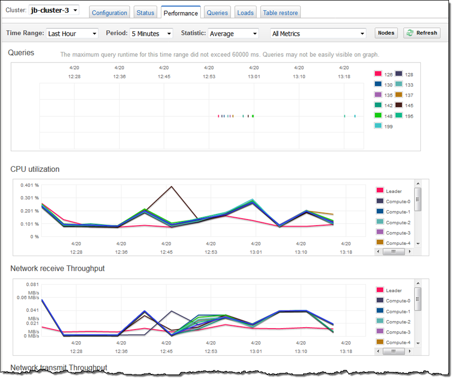
As you can see, Spectrum was able to churn through all 6 billion rows in about 15 seconds. I checked my cluster’s performance metrics and it looked like I had enough CPU power to run many such queries simultaneously:
Available Now
Amazon Redshift Spectrum is available now and you can start using it today!
Spectrum pricing is based on the amount of data pulled from S3 during query processing and is charged at the rate of $5 per terabyte (you can save money by compressing your data and/or storing it in column-oriented form). You pay the usual charges to run your Redshift cluster and to store your data in S3, but there are no Spectrum charges when you are not running queries.
— Jeff;
PS – Several people have asked about the relationship between Spectrum and Athena, and the applicability of both tools to different workloads. Fortunately, the newly updated Redshift FAQ addresses this question; see When should I use Amazon Athena vs. Redshift Spectrum? for more info.
Data Compression Improvements in Amazon Redshift Bring Compression Ratios Up to 4x
Maor Kleider, Senior Product Manager with Amazon Redshift, wrote today’s guest post.
-Ana
Amazon Redshift, is a fast, fully managed, petabyte-scale data warehousing service that makes it simple and cost-effective to analyze all of your data. Many of our customers, including Scholastic, King.com, Electronic Arts, TripAdvisor and Yelp, migrated to Amazon Redshift and achieved agility and faster time to insight, while dramatically reducing costs.
Columnar compression is an important technology in Amazon Redshift. It both helps reduce customer costs by increasing the effective storage capacity of our nodes and improves performance by reducing I/O needed to process SQL requests. Improving I/O efficiency is very important for data warehousing. Last year, our I/O enhancements doubled query throughput. Let’s talk about some of the new compression improvements we’ve recently added to Amazon Redshift.

First, we added support for the Zstandard compression algorithm, which offers a good balance between a high compression ratio and speed in build 1.0.1172. When applied to raw data in the standard TPC-DS, 3 TB benchmark, Zstandard achieves 65% reduction in disk space. Zstandard is broadly applicable. You can apply it to any of the following data types: SMALLINT, INTEGER, BIGINT, DECIMAL, REAL, DOUBLE PRECISION, BOOLEAN, CHAR, VARCHAR, DATE, TIMESTAMP and TIMESTAMPTZ.
Second, we’ve improved the automation of compression on tables created by the CREATE TABLE AS, CREATE TABLE or ALTER TABLE ADD COLUMN commands. Starting with Build 1.0.1161, Amazon Redshift automatically chooses a default compression for the columns created by those commands. Automated compression happens when we estimate that we can reduce disk space without degrading query performance. Our customers have seen up to 40% reduction in disk space.
Third, we’ve been optimizing our internal on-disk data structures. Our preview customers averaged a 7% reduction in disk space usage with this improvement. This feature is delivered starting with Build 1.0.1271.
Finally, we have enhanced the ANALYZE COMPRESSION command to estimate disk space reduction. You can now easily identify opportunities to further compress data and improve performance. Behind the scenes, we sample your data and suggest the most effective compression. You can then specify the recommended encodings or your preferred encodings based on your own evaluation.
“Before all the recent compression features, our largest table was over 7 TB. It’s now only 4.85 TB, which is an additional 30.7% reduction in disk space. This allows us to reduce our disk space by 4X in total and our effective cost to less than $250/TB/Year on an uncompressed data basis. We’re now able to analyze more data with Amazon Redshift, and our query performance has gotten even better.” Chuong Do, Director of Analytics, Coursera
Of course, the actual benefits you see on your clusters will depend upon your workload and your data. In combination, these improvements may reduce your data sets by up to 4x vs. the 3x most of our customers saw before.
You may have heard us talk about how an Amazon Redshift data warehouse can cost as little as $1,000 per terabyte per year. It is important to realize that we’re talking about compressed data in this number. After all, that’s what we store. Not all vendors do this – many compress your data under the covers but describe per-terabyte costs in terms of uncompressed data. That’s unfortunate – the difference between talking in terms of uncompressed data and compressed data can be a significant overstatement.
-Maor Kleider
AWS Database Migration Service – 20,000 Migrations and Counting
I first wrote about AWS Database Migration Service just about a year ago in my AWS Database Migration Service post. At that time I noted that over 1,000 AWS customers had already made use of the service as part of their move to AWS.
As a quick recap, AWS Database Migration Service and Schema Conversion Tool (SCT) help our customers migrate their relational data from expensive, proprietary databases and data warehouses (either on premises on in the cloud, but with restrictive licensing terms either way) to more cost-effective cloud-based databases and data warehouses such as Amazon Aurora, Amazon Redshift, MySQL, MariaDB, and PostgreSQL, with minimal downtime along the way. Our customers tell us that they love the flexibility and the cost-effective nature of these moves. For example, moving to Amazon Aurora gives them access to a database that is MySQL and PostgreSQL compatible, at 1/10th the cost of a commercial database. Take a peek at our AWS Database Migration Services Customer Testimonials to see how Expedia, Thomas Publishing, Pega, and Veoci have made use of the service.
20,000 Unique Migrations
I’m pleased to be able to announce that our customers have already used AWS Database Migration Service to migrate 20,000 unique databases to AWS and that the pace continues to accelerate (we reached 10,000 migrations in September of 2016).
We’ve added many new features to DMS and SCT over the past year. Here’s a summary:
- March 2016 – General availability in eight AWS regions.
- May 2016 – Addition of Redshift as a migration target.
- July 2016 – Highly available architecture for ongoing replication.
- July 2016 – SSL-enabled endpoints & support for Sybase as a migration source and target.
- August 2016 – Expansion to Asia Pacific (Mumbai), Asia Pacific (Seoul), and South America (São Paulo) Regions.
- October 2016 – Expansion to US East (Ohio) Region.
- December 2016 – Support for Oracle SSL connections.
- December 2016 – Expansion to Canada (Central) and EU (London) Regions.
- January 2017 – Support for events and event subscriptions.
- February 2017 – Migration from Oracle and Teradata data warehouses to Amazon Redshift.
Learn More
Here are some resources that will help you to learn more and to get your own migrations underway, starting with some recent webinars:
 Migrating From Sharded to Scale-Up – Some of our customers implemented a scale-out strategy in order to deal with their relational workload, sharding their database across multiple independent pieces, each running on a separate host. As part of their migration, these customers often consolidate two or more shards onto a single Aurora instance, reducing complexity, increasing reliability, and saving money along the way. If you’d like to do this, check out the blog post, webinar recording, and presentation.
Migrating From Oracle or SQL Server to Aurora – Other customers migrate from commercial databases such as Oracle or SQL Server to Aurora. If you would like to do this, check out this presentation and the accompanying webinar recording.
We also have plenty of helpful blog posts on the AWS Database Blog:
- Reduce Resource Consumption by Consolidating Your Sharded System into Aurora – “You might, in fact, save bunches of money by consolidating your sharded system into a single Aurora instance or fewer shards running on Aurora. That is exactly what this blog post is all about.”
- How to Migrate Your Oracle Database to Amazon Aurora – “This blog post gives you a quick overview of how you can use the AWS Schema Conversion Tool (AWS SCT) and AWS Database Migration Service (AWS DMS) to facilitate and simplify migrating your commercial database to Amazon Aurora. In this case, we focus on migrating from Oracle to the MySQL-compatible Amazon Aurora.”
- Cross-Engine Database Replication Using AWS Schema Conversion Tool and AWS Database Migration Service – “AWS SCT makes heterogeneous database migrations easier by automatically converting source database schema. AWS SCT also converts the majority of custom code, including views and functions, to a format compatible with the target database.”
- Database Migration—What Do You Need to Know Before You Start? – “Congratulations! You have convinced your boss or the CIO to move your database to the cloud. Or you are the boss, CIO, or both, and you finally decided to jump on the bandwagon. What you’re trying to do is move your application to the new environment, platform, or technology (aka application modernization), because usually people don’t move databases for fun.”
- How to Script a Database Migration – “You can use the AWS DMS console or the AWS CLI or the AWS SDK to perform the database migration. In this blog post, I will focus on performing the migration with the AWS CLI.”
The documentation includes five helpful walkthroughs:
- Migrating Databases to Amazon Web Services.
- Migrating an On-Premises Oracle Database to Amazon Aurora Using AWS Database Migration Service.
- Migrating an Amazon RDS Oracle Database to Amazon Aurora Using AWS Database Migration Service.
- Migrating MySQL-Compatible Databases to AWS.
- Migrating MySQL-Compatible Databases to Amazon Aurora.
There’s also a hands-on lab (you will need to register in order to participate).
See You at a Summit
The DMS team is planning to attend and present at many of our upcoming AWS Summits and would welcome the opportunity to discuss your database migration requirements in person.
— Jeff;
Amazon Kinesis- Setting up a Streaming Data Pipeline
Ray Zhu from the Amazon Kinesis team wrote this great post about how to set up a streaming data pipeline. He carefully shows you step by step how he set it all up and how you can do it too.
-Ana
Consumer demand for better experiences is ever increasing today. Companies across different industry segments are looking for ways to differentiate their products and services. Data is a key ingredient for providing differentiated products and services, and this is no longer a secret but rather a well adopted practice. Almost all companies at meaningful size are using some sort of data technologies, which means being able to collect and use data is no longer enough as a differentiating factor. Then what? How fast you can collect and use your data becomes the key to stay competitive.
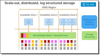
Streaming data technologies shorten the time to analyze and use your data from hours and days to minutes and seconds. Let’s walk through an example of using Amazon Kinesis Firehose, Amazon Redshift, and Amazon QuickSight to set up a streaming data pipeline and visualize Maryland traffic violation data in real time.
Data Flow Overview

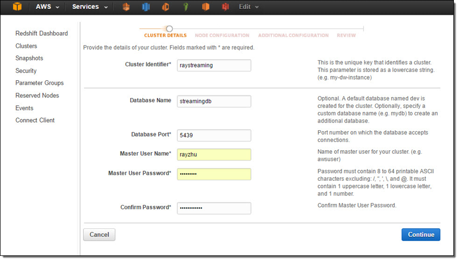
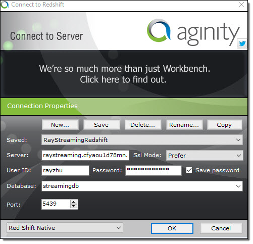
Step 1 Set up Redshift database and table
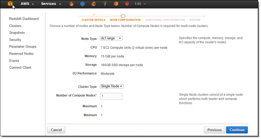
In this step, I’ll set up a Redshift table for Kinesis Firehose to continuously load streaming data into. I first start a single node Redshift cluster and name it “raystreaming.”
Under “Additional Configuration”, I make the cluster publicly accessible so that Kinesis Firehose and QuickSight can connect to my cluster.
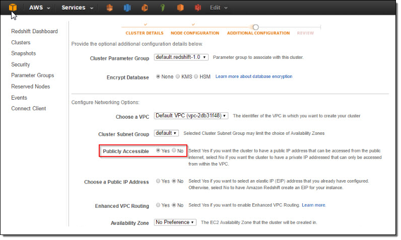
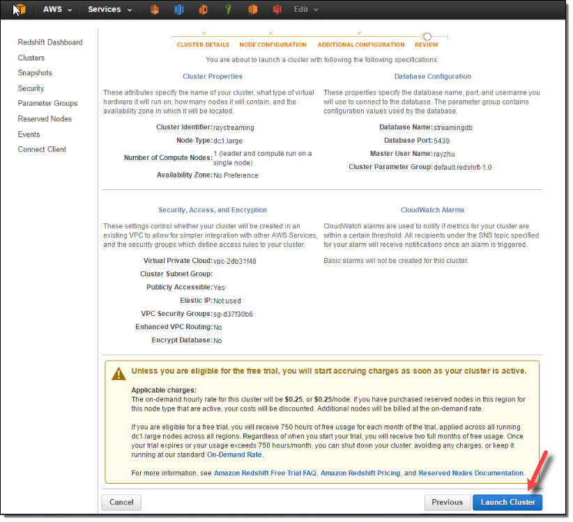
After reviewing all configurations, I click on “Launch Cluster”.
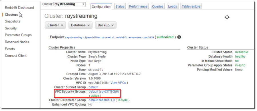
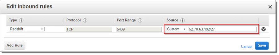
Once the cluster is active, I go to the cluster’s VPC Security Groups to add inbound access for Kinesis Firehose service IPs and outbound access for QuickSight service IPs.
Kinesis Firehose service IPs:
| US East (N. Virginia) | 52.70.63.192/27 |
| US West (Oregon) | 52.89.255.224/27 |
| EU (Ireland) | 52.19.239.192/27 |
QuickSight service IPs:
| US East (N. Virginia) | 52.23.63.224/27 |
| US West (Oregon) (us-west-2) | 54.70.204.128/27 |
| EU (Ireland) (eu-west-1) | 52.210.255.224/27 |
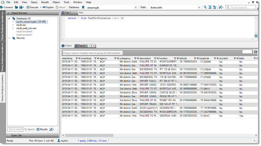
Now the cluster is setup and configured. I’ll use a JDBC tool and the SQL statement below to create a table for storing Maryland traffic violation data.
create table TrafficViolation(
 dateofstop date,
 timeofstop timestamp,
 agency varchar(100),
 subagency varchar(100),
 description varchar(300),
 location varchar(100),
 latitude varchar(100),
 longtitude varchar(100),
 accident varchar(100),
 belts varchar(100),
 personalinjury varchar(100),
 propertydamage varchar(100),
 fatal varchar(100),
 commlicense varchar(100),
 hazmat varchar(100),
 commvehicle varchar(100),
 alcohol varchar(100),
 workzone varchar(100),
 state varchar(100),
 veichletype varchar(100),
 year varchar(100),
 make varchar(100),
 model varchar(100),
 color varchar(100),
 violation varchar(100),
 type varchar(100),
 charge varchar(100),
 article varchar(100),
 contributed varchar(100),
 race varchar(100),
 gender varchar(100),
 drivercity varchar(100),
 driverstate varchar(100),
 dlstate varchar(100),
 arresttype varchar(100),
 geolocation varchar(100));
Step 2 Set up Kinesis Firehose delivery stream
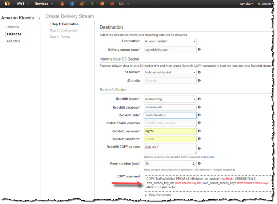
In this step, I’ll set up a Kinesis Firehose delivery stream to continuously deliver data to the “TrafficViolation” table created above.
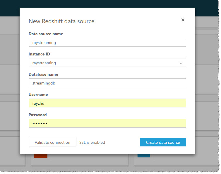
I name my Firehose delivery stream “rayredshiftstream”. Under destination configurations, I choose “Amazon Redshift” as destination and configure an intermediate S3 bucket. Kinesis Firehose will first load my streaming data to this intermediate buckets and then COPY it to Redshift. Loading data from S3 to Redshift is efficient and preserves resources on Redshift for queries. Also, I always have a backup of my data in S3 for other batch processes or in case my Redshift cluster is not accessible (e.g. under maintenance).
Subsequently, I enter the Redshift cluster, database, and table names along with Redshift user name and password. This user needs to have Redshift INSERT permission. I also specify “json ‘auto’” under COPY options to parse JSON formatted sample data.
I set retry duration to 30 seconds. In cases when data load to my Redshift cluster fails, Kinesis Firehose will retry for 30 seconds. The failed data is always in the intermediate S3 bucket for backfill. At the bottom, the exact COPY command Kinesis Firehose will use is generated for testing purposes.
On the next page, I specify buffer size and buffer interval. Kinesis Firehose buffers streaming data to a certain size or for a certain period of time before loading it to S3. Kinesis Firehose’s buffering feature reduces S3 PUT requests and cost significantly and generates relatively larger S3 object size for efficient data load to Redshift. I’m using the smallest buffer size (1MB) and shortest buffer interval (60 seconds) in this example in order to have data delivered sooner.
You can also optionally configure Kinesis Firehose to compress the data in GZIP format before loading it to S3 and use a KMS key to encrypt the data in S3. In this example, I configure my data to be uncompressed and unencrypted. Please note that if you enable GZIP compression, you’ll also need to add “gzip” under Redshift COPY options.
I also enable error logging for Kinesis Firehose to log any delivery errors to my CloudWatch Log group. The error messages are viewable from Kinesis Firehose console as well and are particularly useful for troubleshooting purpose.
Finally, I configure a default IAM role to allow Kinesis Firehose to access the resources I configured in the delivery stream.
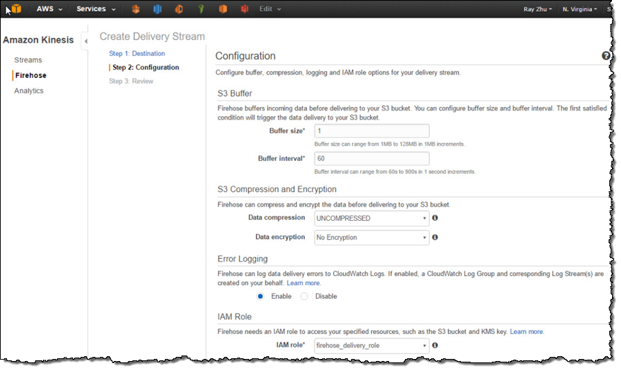
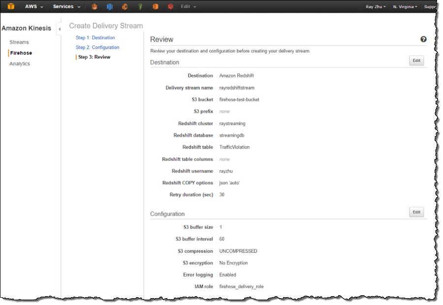
After reviewing all configurations, I click on “Create Delivery Stream”.
Step 3 Send data to Kinesis Firehose delivery stream
Now my Firehose delivery stream is set up and pointing to my Redshift table “TrafficViolation”. In this example, I’m using the Traffic Violations dataset from US Government Open Data. I use the Kinesis Firehose sample from AWS Java SDK to parse records from local csv file and send each record to my delivery stream.
In real streaming use cases, you can imagine that each data record is pushed to the delivery stream from police officer’s cellular devices through Firehose’s PutRecord() or PutRecordBatch() APIs as soon as a violation ticket is recorded.
A sample of the data looks like the following and includes information such as time of stop, vehicle type, driver gender, and so forth.
09/30/2014,23:51:00,MCP,"1st district, Rockville",\
  DRIVER FAILURE TO STOP AT STEADY CIRCULAR RED SIGNAL,\
  PARK RD AT HUNGERFORD DR,,,No,No,No,No,No,No,No,No,No,No,\
  MD,02 - Automobile,2014,FORD,MUSTANG,BLACK,Citation,21-202(h1),\
  Transportation Article,No,BLACK,M,ROCKVILLE,MD,MD,A - Marked Patrol,
Step 4 Visualize the data from QuickSight
As I continuously push data records to my delivery stream “rayredshiftstream”, I can see these data gets populated to my Redshift table “TrafficViolation” continuously.
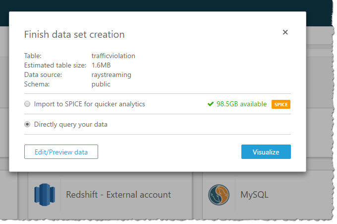
Now I’m going to use QuickSight to analyze and visualize the data from my Redshift table “TrafficViolation”. I create a new analysis and a new data set pointing to my Redshift table “TrafficViolation”.
I use “Query” mode to directly retrieve data from my Redshift cluster so that new data is retrieved as they are continuously streamed from Kinesis Firehose.
With a few clicks, I create a bar chart graph that displays number of traffic violations by gender and hour of the day. There are a few interesting patterns: 1) Male drivers have significantly more traffic violations than female drivers during morning hours. 2) Noon has the lowest number of violations. 3) From 2pm to 4pm, the number of violations gap between male and female drivers narrows.
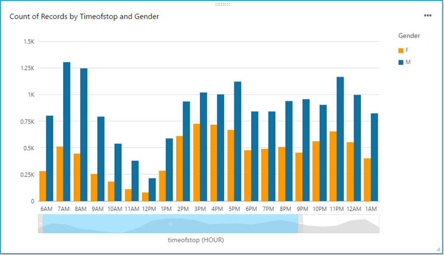
With a live dashboard, this graph will keep updating itself throughout the day as new data continuously gets streamed from police officer’s devices to Redshift through Kinesis Firehose. Another interesting live dashboard to build will be a map graph that shows a heat map of traffic violations across different districts of Maryland over time. I’ll leave this exercise to the readers of this blog and you can use your favorite Business Intelligent tools to do so.
That’s it!
Hopefully through reading this blog and trying it out yourself, you’ve got some inspirations about streaming data and a sense of how easy it is to get started with streaming data analytics on AWS. I cannot wait to see what streaming data analytics pipelines and applications you can build for your organizations!
-Ray Zhu
Amazon QuickSight Now Generally Available – Fast & Easy to Use Business Analytics for Big Data
 After a preview period that included participants from over 1,500 AWS customers ranging from startups to global enterprises, I am happy to be able to announce that Amazon QuickSight is now generally available! When I invited you to join the preview last year, I wrote:
In the past, Business Intelligence required an incredible amount of undifferentiated heavy lifting. You had to pay for, set up and run the infrastructure and the software, manage scale (while users fret), and hire consultants at exorbitant rates to model your data. After all that your users were left to struggle with complex user interfaces for data exploration while simultaneously demanding support for their mobile devices. Access to NoSQL and streaming data? Good luck with that!
Amazon QuickSight provides you with very fast, easy to use, cloud-powered business analytics at 1/10th the cost of traditional on-premises solutions. QuickSight lets you get started in minutes. You log in, point to a data source, and begin to visualize your data. Behind the scenes, the SPICE (Super-fast, Parallel, In-Memory Calculation Engine) will run your queries at lightning speed and provide you with highly polished data visualizations.
Deep Dive into Data
Every customer that I speak with wants to get more value from their stored data. They realize that the potential value locked up within the data is growing by the day, but are sometimes disappointed to learn that finding and unlocking that value can be expensive and difficult. On-premises business analytics tools are expensive to license and can place a heavy load on existing infrastructure. Licensing costs and the complexity of the tools can restrict the user base to just a handful of specialists. Taken together, all of these factors have led many organizations to conclude that they are not ready to make the investment in a true business analytics function.
QuickSight is here to change that! It runs as a service and makes business analytics available to organizations of all shapes and sizes. It is fast and easy to use, does not impose a load on your existing infrastructure, and is available for a monthly fee that starts at just $9 per user.
As you’ll see in a moment, QuickSight allows you to work on data that’s stored in many different services and locations. You can get to your Amazon Redshift data warehouse, your Amazon Relational Database Service (RDS) relational databases, or your flat files in S3. You can also use a set of connectors to access data stored in on-premises MySQL, PostgreSQL, and SQL Server databases, Microsoft Excel spreadsheets, Salesforce and other services.
QuickSight is designed to scale with you. You can add more users, more data sources, and more data without having to purchase more long-term licenses or roll more hardware into your data center.
Take the Tour
Let’s take a tour through QuickSight. The administrator for my organization has already invited me to use QuickSight, so I am ready to log in and get started. Here’s the main screen:
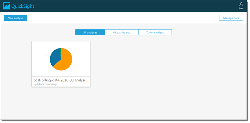
I’d like to start by getting some data from a Redshift cluster. I click on Manage data and review my existing data sets:
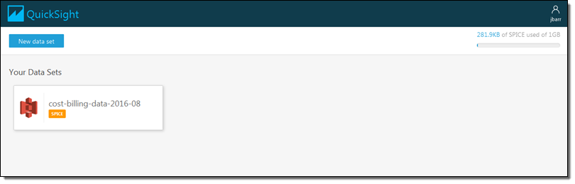
I don’t see what I am looking for, so I click on New data set and review my options:
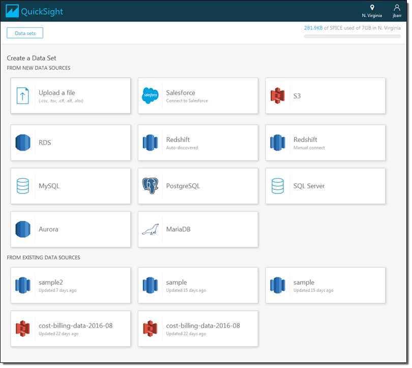
I click on Redshift (manual connect) and enter the credentials so that I can access my data warehouse (if I had a Redshift cluster running within my AWS account it would be available as an auto-discovered source):
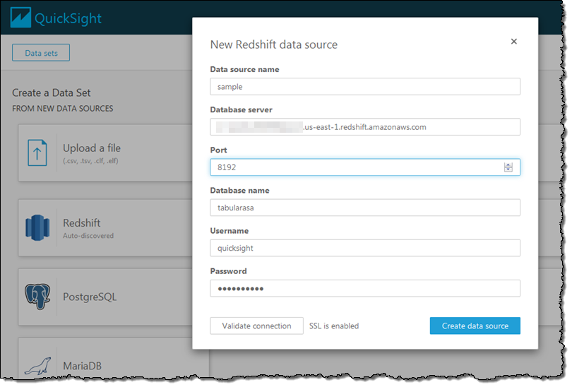
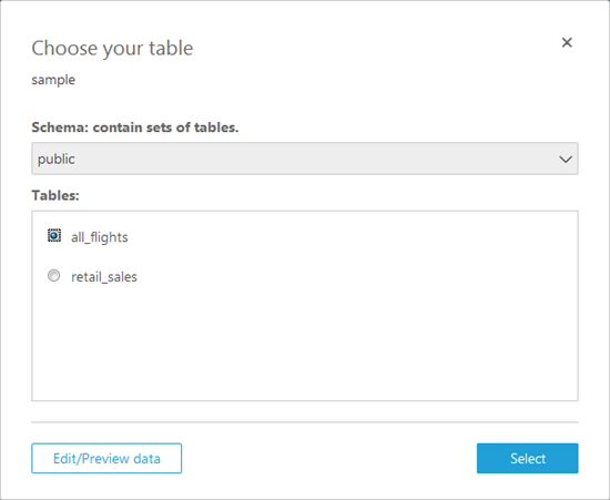
QuickSight queries the data warehouse and shows me the schemas (sets of tables) and the tables that are available to me. I’ll select the public schema and the all_flights table to get started:
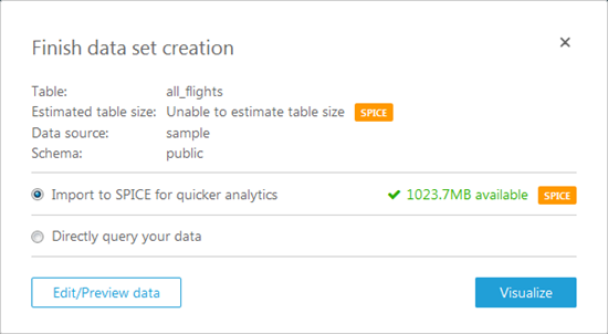
Now I have two options. I can pull the table in to SPICE for quick analysis or I can query it directly. I’ll pull it in to SPICE:
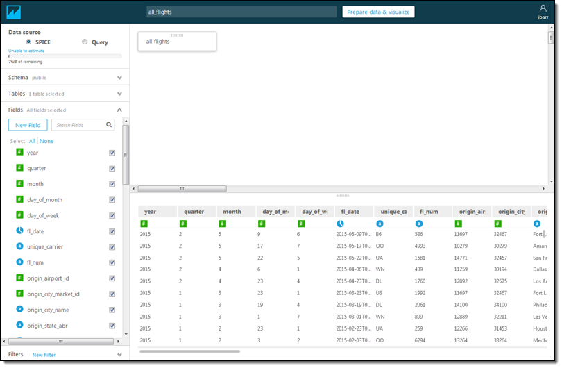
Again, I have two options! I can click on Edit/Preview data and select the rows and columns to import, or I can click on Visualize to import all of the data and proceed to the fun part! I’ll go for Edit/Preview. I can see the fields (on the left), and I can select only those that are interest using the checkboxes:
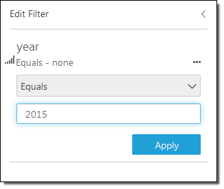
I can also click on New Filter, select a field from the popup menu, and then create a filter:
Both options (selecting fields and filtering on rows) allow me to control the data that I pull in to SPICE. This allows me to control the data that I want to visualize and also helps me to make more efficient use of memory. Once I am ready to proceed, I click on Prepare data & visualize. At this point the data is loaded in to SPICE and I’m ready to start visualizing it. I simply select a field to get started. For example, I can select the origin_state_abbr field and see how many flights originate in each state:
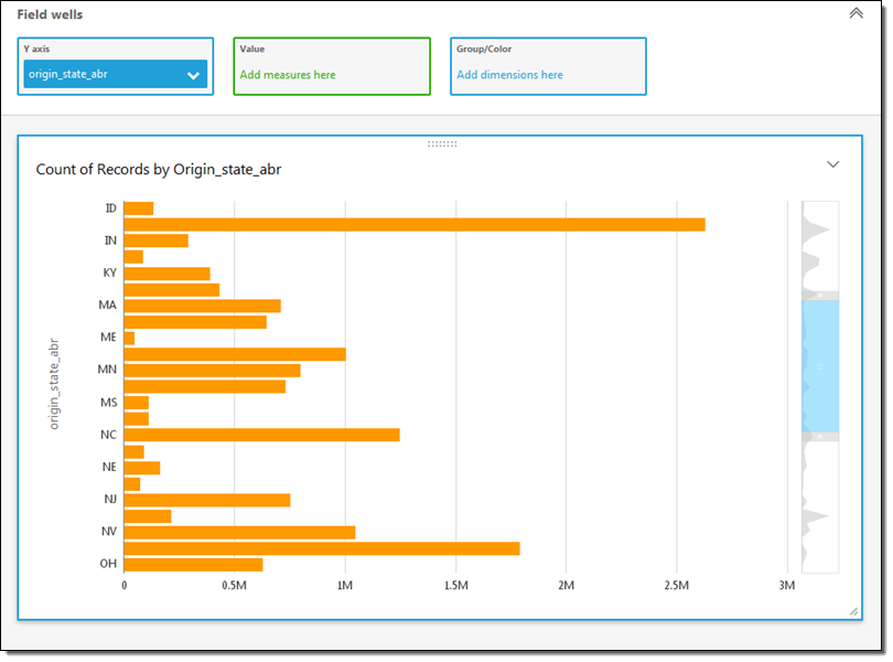
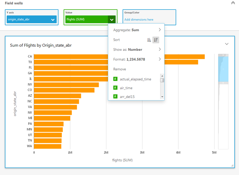
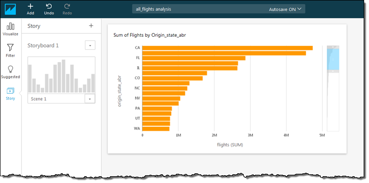
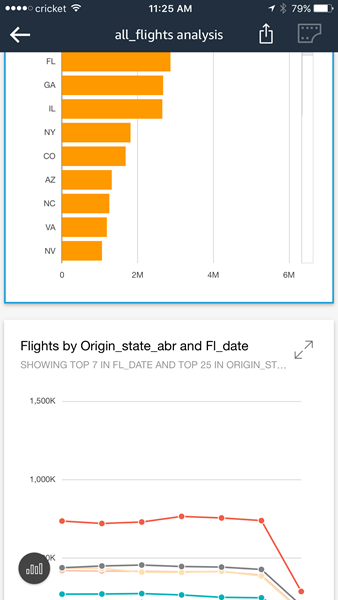
The miniaturized view on the right gives me some additional context. I can scroll up or down or select the range of values to display. I can also click on a second field to learn more. I’ll click on flights, set the sort order to descending, and scroll to the top. Now I can see how many of the flights in my data originated in each state:
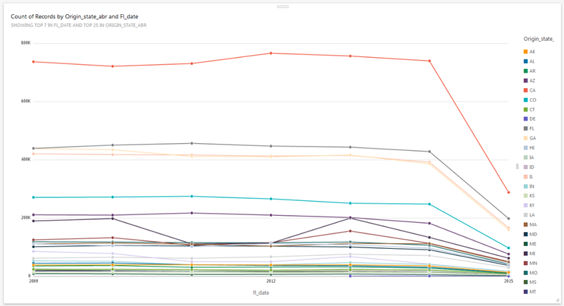
QuickSight’s AutoGraph feature automatically generates an appropriate visualization based on the data selected. For example, if I add the fl_date field, I get a state-by-state line chart over time:
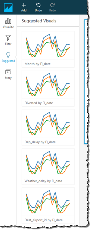
Based on my query, the data types, and properties of the data, QuickSight also proposes alternate visualizations:
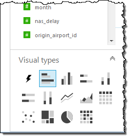
I also have my choice of many other visual types including vertical & horizontal bar charts, line charts, pivot tables, tree maps, pie charts, and heat maps:
Once I have created some effective visualizations, I can capture them and use the resulting storyboard to tell a data-driven story:
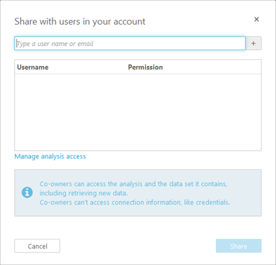
I can also share my visualizations with my colleagues:
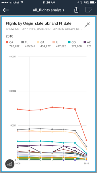
Finally, my visualizations are accessible from my mobile device:
Pricing & SPICE Capacity
QuickSight comes with one free user and 1 GB of SPICE capacity for free, perpetually. This allows every AWS user to analyze their data and to gain business insights at no cost. The Standard Edition of Amazon QuickSight starts at $9 per month and includes 10 GB of SPICE capacity (see the [QuickSight Pricing] page for more info).
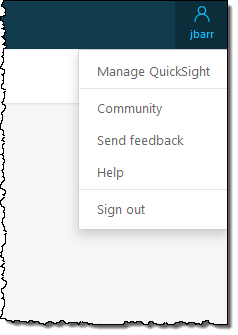
It is easy to manage SPICE capacity. I simply click on Manage QuickSight in the menu (I must have the ADMIN role in order to be able to make changes):
Then I can see where I stand:
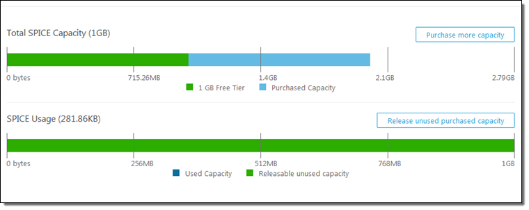
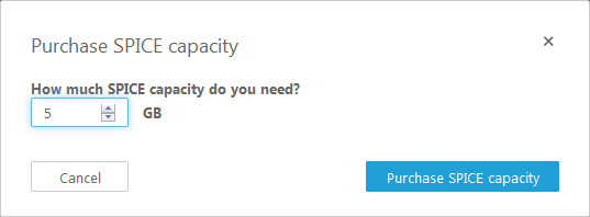
I can click on Purchase more capacity to do exactly that:
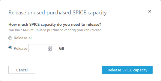
I can also click on Release unused purchased capacity in order to reduce the amount of SPICE capacity that I own:
Get Started Today
Amazon QuickSight is now available in the US East (Northern Virginia), US West (Oregon), and EU (Ireland) regions and you can start using it today.
Despite the length of this blog post I have barely scratched the surface of QuickSight. Given that you can use it at no charge, I would encourage you to sign up, load some of your data, and take QuickSight for a spin!
We have a webinar coming up on January 16th where you can learn even more! Sign up here.
— Jeff;
New – Upload AWS Cost & Usage Reports to Redshift and QuickSight
Many AWS customers have been asking us for a way to programmatically analyze their Cost and Usage Reports (read New – AWS Cost and Usage Reports for Comprehensive and Customizable Reporting for more info). These customers are often using AWS to run multiple lines of business, making use of a wide variety of services, often spread out across multiple regions. Because we provide very detailed billing and cost information, this is a Big Data problem and one that can be easily addressed using AWS services!
While I was on vacation earlier this month, we launched a new feature that allows you to upload your Cost and Usage reports to Amazon Redshift and Amazon QuickSight. Now that I am caught up, I’d like to tell you about this feature.
Upload to Redshift
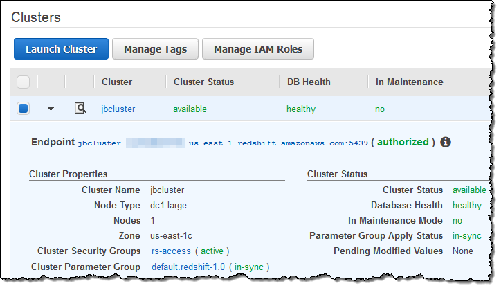
I started by creating a new Redshift cluster (if you already have a running cluster, you need not create another one). Here’s my cluster:
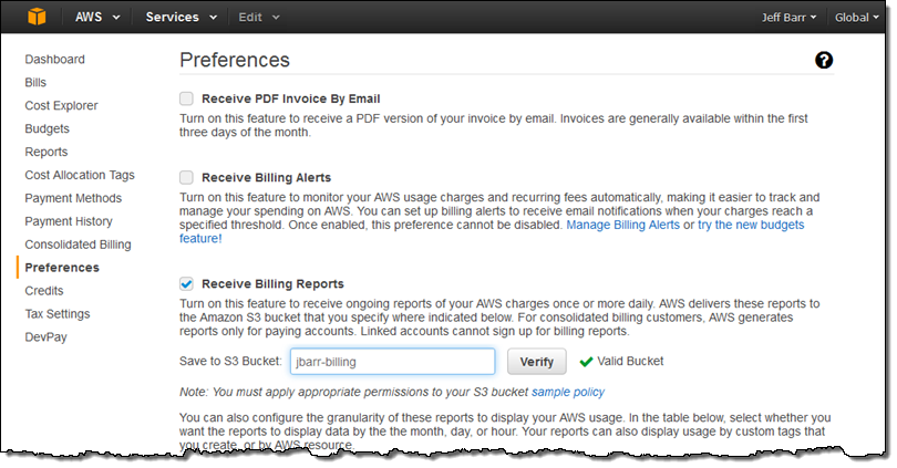
Next, I verified that I had enabled the Billing Reports feature:
Then I hopped over to the Cost and Billing Reports and clicked on Create report:
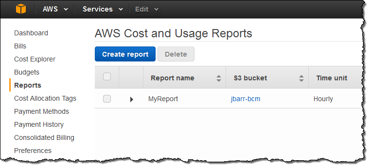
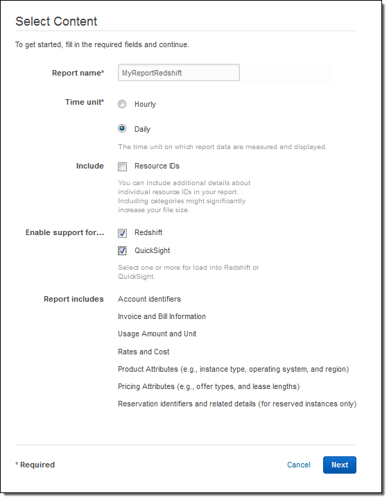
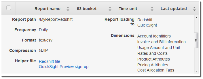
Next, I named my report (MyReportRedshift), made it Hourly, and enabled support for both Redshift and QuickSight:
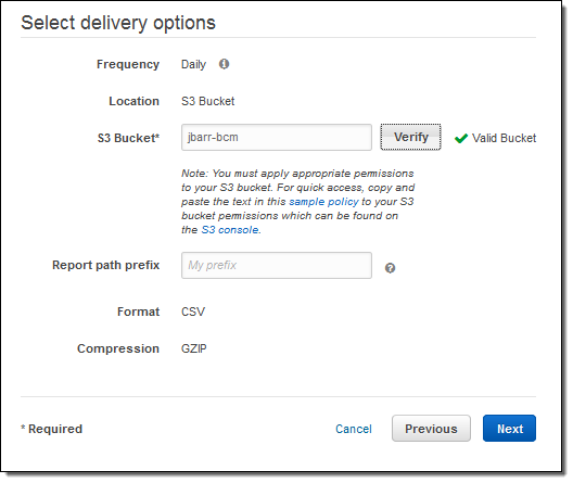
I wrapped things up by selecting my delivery options:
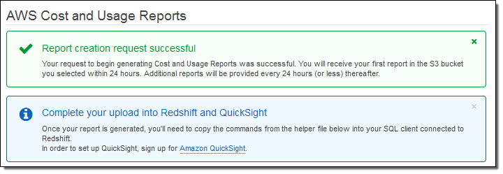
I confirmed my desire to create a report on the next page, and then clicked on Review and Complete. The report was created and I was informed that the first report would arrive in the bucket within 24 hours:
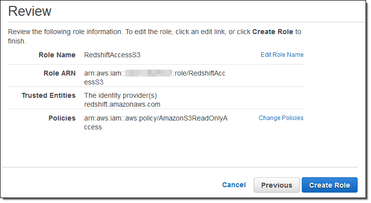
While I was waiting I installed PostgreSQL on my EC2 instance (sudo yum install postgresql94) and verified that I was signed up for the Amazon QuickSight preview. Also, following the directions in Create an IAM Role, I made a read-only IAM role and captured its ARN:
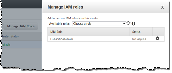
Back in the Redshift console, I clicked on Manage IAM Roles and associated the ARN with my Redshift cluster:
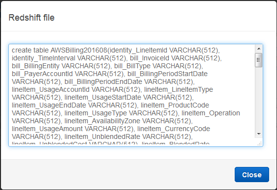
The next day, I verified that the files were arriving in my bucket as expected, and then returned to the console in order to retrieve a helper file so that I could access Redshift:
I clicked on Redshift file and then copied the SQL command:
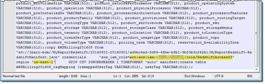
I inserted the ARN and the S3 region name into the SQL (I had to add quotes around the region name in order to make the query work as expected):
And then I connected to Redshift using psql (I can use any visual or CLI-based SQL client):
$ psql -h jbcluster.XYZ.us-east-1.redshift.amazonaws.com \
  -U root -p 5439 -d dev
Then I ran the SQL command. It created a pair of tables and imported the billing data from S3.
Querying Data in Redshift
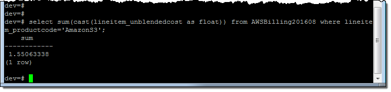
Using some queries supplied by my colleagues as a starting point, I summed up my S3 usage for the month:
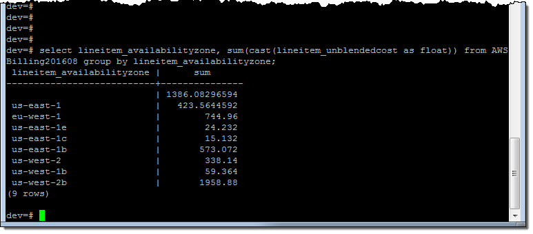
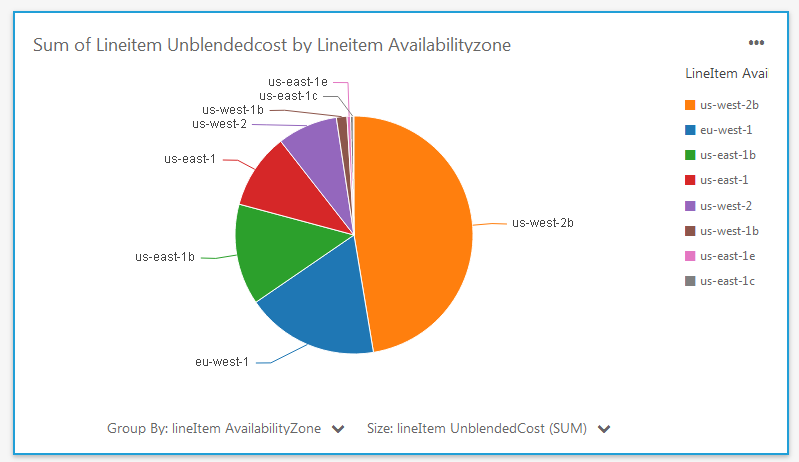
And then I looked at my costs on a per-AZ basis:
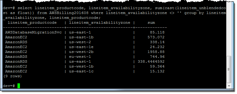
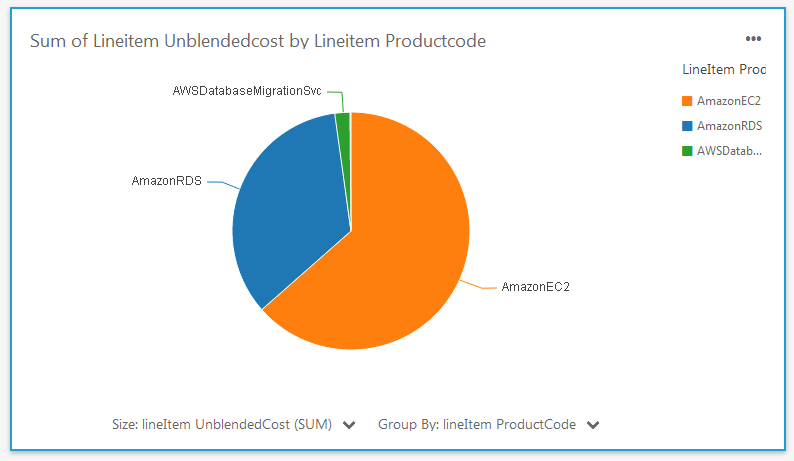
And on a per-AZ, per-service basis:
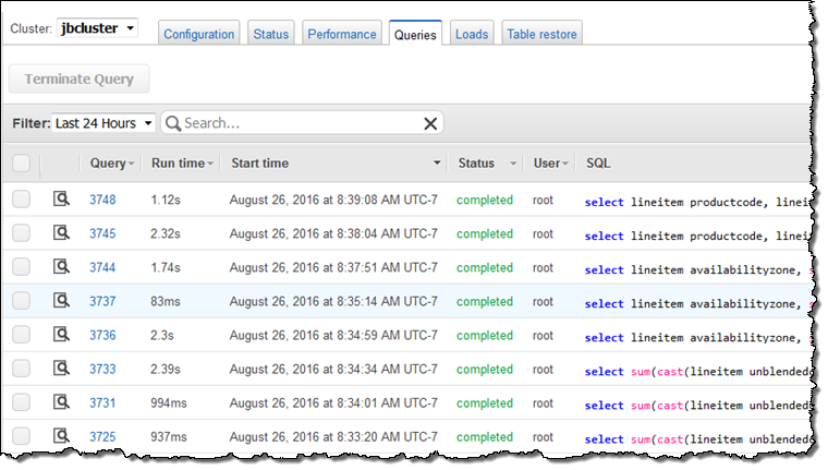
 Just for fun, I spent some time examining the Redshift Console. I was able to see all of my queries:
Analyzing Data with QuickSight
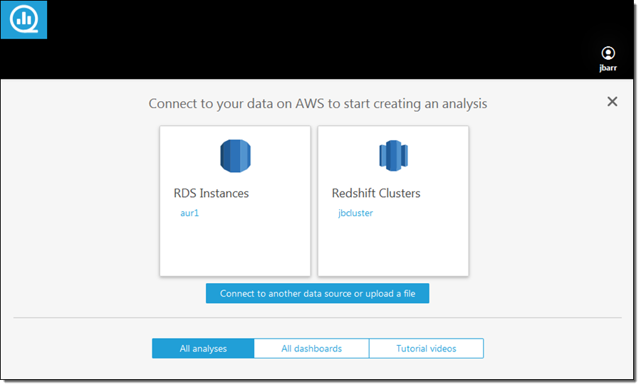
I also spent some time analyzing the cost and billing data using Amazon QuickSight. I signed in and clicked on Connect to another data source or upload a file:
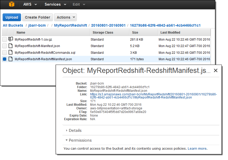
Then I dug in to my S3 bucket (jbarr-bcm) and captured the URL of the manifest file (MyReportRedshift-RedshiftManifest.json):
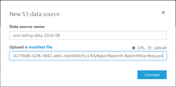
I selected S3 as my data source and entered the URL:
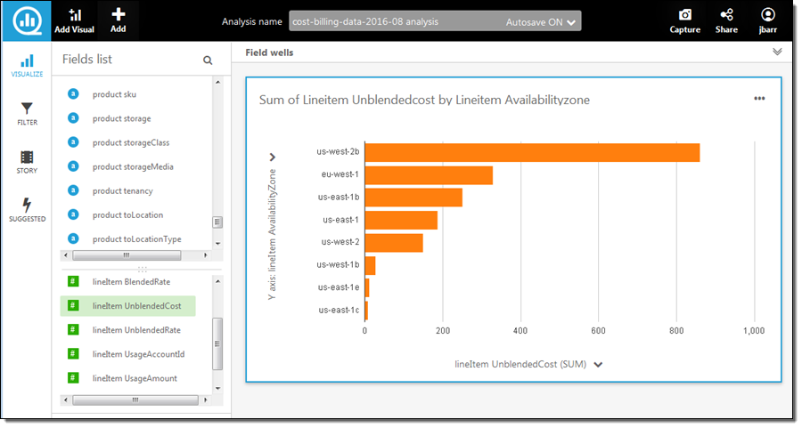
QuickSight imported the data in a few seconds and the new data source was available. I loaded it into SPICE (QuickSight’s in-memory calculation engine). With three or four more clicks I focused on the per-AZ data, and excluded the data that was not specific to an AZ:
Another click and I switched to a pie chart view:
I also examined the costs on a per-service basis:
As you can see, the new data and the analytical capabilities of QuickSight allow me (and you) to dive deep into your AWS costs in minutes.
Available Now
This new feature is available now and you can start using it today!
— Jeff;
Learn about Amazon Redshift in our new Data Warehousing on AWS Class
 As our customers continue to look to use their data to help drive their missions forward, finding a way to simply and cost-effectively make use of analytics is becoming increasingly important. That is why I am happy to announce the upcoming availability of Data Warehousing on AWS, a new course that helps customers leverage the AWS Cloud as a platform for data warehousing solutions.
New Course
Data Warehousing on AWS is a new three-day course that is designed for database architects, database administrators, database developers, and data analysts/scientists. It introduces you to concepts, strategies, and best practices for designing a cloud-based data warehousing solution using Amazon Redshift. This course demonstrates how to collect, store, and prepare data for the data warehouse by using other AWS services such as Amazon DynamoDB, Amazon EMR, Amazon Kinesis, and Amazon S3. Additionally, this course demonstrates how you can use business intelligence tools to perform analysis on your data. Organizations who are looking to get more out of their data by implementing a Data Warehousing solution or expanding their current Data Warehousing practice are encouraged to sign up.
These classes (and many more) are available through AWS and our Trainintg Partners. Find upcoming classes in our global training schedule or learn more at AWS Training.
— Jeff;
Amazon Redshift – Up to 2X Throughput and 10X Vacuuming Performance Improvements
My colleague Maor Kleider wrote today’s guest post!
— Jeff;
Amazon Redshift, AWS’s fully managed data warehouse service, makes petabyte-scale data analysis fast, cheap, and simple. Since launch, it has been one of AWS’s fastest growing services, with many thousands of customers across many industries. Enterprises such as NTT DOCOMO, NASDAQ, FINRA, Johnson & Johnson, Hearst, Amgen, and web-scale companies such as Yelp, Foursquare and Yahoo! have made Amazon Redshift a key component of their analytics infrastructure.
In this blog post, we look at performance improvements we’ve made over the last several months to Amazon Redshift, improving throughput by more than 2X and vacuuming performance by 10X.
Column Store
Large scale data warehousing is largely an I/O problem, and Amazon Redshift uses a distributed columnar architecture to minimize and parallelize I/O. In a column-store, each column of a table is stored in its own data block. This reduces data size, since we can choose compression algorithms optimized for each type of column. It also reduces I/O time during queries, because only the columns in the table that are being selected need to be retrieved.
However, while a column-store is very efficient at reading data, it is less efficient than a row-store at loading and committing data, particularly for small data sets. In patch 1.0.1012 (December 17, 2015), we released a significant improvement to our I/O and commit logic. This helped with small data loads and queries using temporary tables. While the improvements are workload-dependent, we estimate the typical customer saw a 35% improvement in overall throughput.
 Regarding this feature, Naeem Ali, Director of Software Development, Data Science at Cablevision, told us:
Following the release of the I/O and commit logic enhancement, we saw a 2X performance improvement on a wide variety of workloads. The more complex the queries, the higher the performance improvement.
Improved Query Processing
In addition to enhancing the I/O and commit logic for Amazon Redshift, we released an improvement to the memory allocation for query processing in patch 1.0.1056 (May 17, 2016), increasing overall throughput by up to 60% (as measured on standard benchmarks TPC-DS, 3TB), depending on the workload and the number of queries that spill from memory to disk. The query throughput improvement increases with the number of concurrent queries, as less data is spilled from memory to disk, reducing required I/O.
Taken together, these two improvements, should double performance for customer workloads where a portion of the workload contains complex queries that spill to disk or cause temporary tables to be created.
Better Vacuuming
Amazon Redshift uses multi-version concurrency control to reduce contention between readers and writers to a table. Like PostgreSQL, it does this by marking old versions of data as deleted and new versions as inserted, using the transaction ID as a marker. This allows readers to build a snapshot of the data they are allowed to see and traverse the table without locking. One issue with this approach is the system becomes slower over time, requiring a vacuum command to reclaim the space. This command reclaims the space from deleted rows and ensures new data that has been added to the table is placed in the right sorted order.
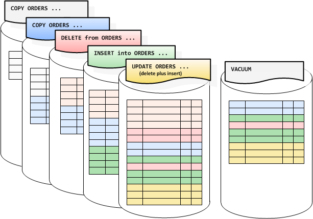
We are releasing a significant performance improvement to vacuum in patch 1.0.1056, available starting May 17, 2016. Customers previewing the feature have seen dramatic improvements both in vacuum performance and overall system throughput as vacuum requires less resources.
 Ari Miller, a Principal Software Engineer at TripAdvisor, told me:
We estimate that the vacuum operation on a 15TB table went about 10X faster with the recent patch, ultimately improving overall query performance.
Available Now
Unlike on-premise data warehousing solutions, there are no license or maintenance fees for these improvements or work required on your part to obtain them. They simply show up as part of the automated patching process during your maintenance window.
— Maor Kleider, Senior Product Manager, Amazon Redshift
User Defined Functions for Amazon Redshift
The Amazon Redshift team is on a tear. They are listening to customer feedback and rolling out new features all the time! Below you will find an announcement of another powerful and highly anticipated new feature.
— Jeff;
Amazon Redshift makes it easy to launch a petabyte-scale data warehouse. For less than $1,000/Terabyte/year, you can focus on your analytics, while Amazon Redshift manages the infrastructure for you. Amazon Redshift’s price and performance has allowed customers to unlock diverse analytical use cases to help them understand their business. As you can see from blog posts by Yelp, Amplitude and Cake, our customers are constantly pushing the boundaries of what’s possible with data warehousing at scale.
To extend Amazon Redshift’s capabilities even further and make it easier for our customers to drive new insights, I am happy to announce that Amazon Redshift has added scalar user-defined functions (UDFs). Using PostgreSQL syntax, you can now create scalar functions in Python 2.7 custom-built for your use case, and execute them in parallel across your cluster.
Here’s a template that you can use to create your own functions:
CREATE [ OR REPLACE ] FUNCTION f_function_name
( [ argument_name arg_type, ... ] )
RETURNS data_type
{ VOLATILE | STABLE | IMMUTABLE }
AS $$
  python_program
$$ LANGUAGE plpythonu;
Scalar UDFs return a single result value for each input value, similar to built-in scalar functions such as ROUND and SUBSTRING. Once defined, you can use UDFs in any SQL statement, just as you would use our built-in functions.
In addition to creating your own functions, you can take advantage of thousands of functions available through Python libraries to perform operations not easily expressed in SQL. You can even add custom libraries directly from S3 and the web. Out of the box, Amazon Redshift UDFs come integrated with the Python Standard Library and a number of other libraries, including:
- NumPy and SciPy, which provide mathematical tools you can use to create multi-dimensional objects, do matrix operations, build optimization algorithms, and run statistical analyses.
- Pandas, which offers high level data manipulation tools built on top of NumPy and SciPy, and that enables you to perform data analysis or an end-to-end modeling workflow.
- Dateutil and Pytz, which make it easy to manipulate dates and time zones (such as figuring out how many months are left before the next Easter that occurs in a leap year).
UDFs can be used to simplify complex operations. For example, if you wanted to extract the hostname out of a URL, you could use a regular expression such as:
SELECT REGEXP_REPLACE(url, '(https?)://([^@]*@)?([^:/]*)([/:].*|$)', ‘\3') FROM table;
Or, you could import a Python URL parsing library, URLParse, and create a function that extracts hostnames:
CREATE FUNCTION f_hostname(url VARCHAR)
RETURNS varchar
IMMUTABLE AS $$
import urlparse
return urlparse.urlparse(url).hostname
$$ LANGUAGE plpythonu;
Now, in SQL all you have to do is:
SELECT f_hostname(url)
FROM table;
As our customers know, Amazon Redshift obsesses about security. We run UDFs inside a restricted container that is fully isolated. This means UDFs cannot corrupt your cluster or negatively impact its performance. Also, functions that write files or access the network are not supported. Despite being tightly managed, UDFs leverage Amazon Redshift’s MPP capabilities, including being executed in parallel on each node of your cluster for optimal performance.
To learn more about creating and using UDFs, please see our documentation and a detailed post on the AWS Big Data blog. Also, check out this how-to guide from APN Partner Looker. If you’d like to share the UDFs you’ve created with other Amazon Redshift customers, please reach out to us at redshift-feedback@amazon.com. APN Partner Periscope has already created a number of useful scalar UDFs and published them here.
We will be patching your cluster with UDFs over the next two weeks, depending on your region and maintenance window setting. The new cluster version will be 1.0.991. We know you’ve been asking for UDFs for some time and would like to thank you for your patience. We look forward to hearing from you about your experience at redshift-feedback@amazon.com.
— Tina Adams, Senior Product Manager
Amazon Redshift – Now Faster and More Cost-Effective than Ever
My colleague Tina Adams sent me a guest post to share news of a new instance type and new Reserved Instance offerings for Amazon Redshift.
— Jeff;
Amazon Redshift makes analyzing petabyte-scale data fast, cheap, and simple. It delivers advanced technology capabilities, including parallel execution, compressed columnar storage, and end-to-end encryption, as a fully managed service, letting you focus on your data not your database. All for less than $1,000/TB/YR. When launching a cluster, you can choose between our Dense Compute (SSD) and Dense Storage (HDD) instance families.
Today, we are making our Dense Storage family even faster and more cost effective with a second-generation instance type, DS2. Moreover, you can now reserve all dense storage and dense compute instances types for one year with No Upfront payment, and receive a 20% discount over On-Demand rates. For steeper discounts, you can pay for your entire reserved instance term with one All Upfront payment.
New DS2 Instances
DS2 instances have twice the memory and compute power of their Dense Storage predecessor, DS1 (previously called DW1), but the same storage. DS2 also supports Enhanced Networking and provides 50% more disk throughput than DS1. On average, DS2 provides 50% better performance than DS1, but is priced exactly the same.
| Instance | vCPU | Memory (GiB)
|
Network | Storage | I/O | Price/TB/Year (On Demand)
|
Price/TB/Year (3 Year RI)
|
| Dense Storage – Current Generation
|
|||||||
| ds2.xlarge | 4 | 31 | Enhanced | 2 TB HDD | 0.50 GBps | $3,330 | $999 |
| ds2.8xlarge | 36 | 244 | Enhanced – 10 Gbps | 16 TB HDD | 4.00 GBps | $3,330 | $999 |
| Dense Storage – Previous Generation (formerly DW1)
|
|||||||
| ds1.xlarge | 2 | 15 | Moderate | 2 TB HDD | 0.30 GBps | $3,330 | $999 |
| ds1.8xlarge | 16 | 120 | 10 Gbps | 16 TB HDD | 2.40 GBps | $3,330 | $999 |
| Dense Compute – Current Generation (formerly DW2) | |||||||
| dc1.large | 2 | 15 | Enhanced | 0.16 TB SSD | 0.20 GBps | $18,327 | $5,498 |
| dc1.8xlarge | 32 | 244 | Enhanced 10 Gbps | 2.56 TB SSD | 3.70 GBps | $18,327 | $5,498 |
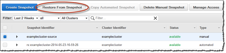
We expect existing DS1 customers to quickly adopt DS2. There’s really no reason not to. To move from DS1 to DS2, simply restore a DS2 cluster from a snapshot of a DS1 cluster of the same size. Restoring from snapshot is a push-button operation in our Console. Our streaming restore feature allows you to resume querying as soon as your new cluster is created, while data is streamed from S3 in the background. After the restore completes, if you’d like, you can resize your DS2 cluster with a few clicks:
No Upfront and All Upfront Reserved Instances
You now have three Reserved Instance payment options! This gives you the flexibility to determine how much you wish to pay upfront. To purchase these offerings simply visit the Reserved Nodes tab in our Console. Here are your options:
No Upfront – You pay nothing upfront, and commit to pay hourly over the course of one year at a 20% discount over On-Demand. This option is only offered for a one year term.
Partial Upfront – The same as our previous heavy utilization RI offering. You pay a portion of the Reserved Instance upfront, and the remainder over a one or three year term. The discount over On-Demand remains at up to 41% for a one year term and up to 73% for a three year term.
All Upfront – You pay for the entire Reserved Instance term (one or three years) with one upfront payment. This is your cheapest option, with a discount of up to 42% for a one year term and up to 76% for a three year term compared to On-Demand.
Stay Tuned
There’s more to come from Amazon Redshift, so stay tuned. To get the latest feature announcements, log in to the Amazon Redshift Forum and subscribe to the Amazon Redshift Announcements thread. Or use the Developer Guide History and the Management Guide History to track product updates. We’d also appreciate your feedback at redshift-feedback@amazon.com.
— Tina Adams, Senior Product Manager